Polarisation purity and beam shapes for the ATCA 16cm receivers
Abstract
The Australia Telescope Compact Array has recently undergone a major upgrade that
has allowed the full bandwidth of the Compact Array Broadband Backend (CABB) to
be utilised at low frequencies. The upgraded 16cm receivers have a usable frequency
range of 1100 - 3100 MHz. This memo investigates the polarisation properties and
beam shapes for this receiver across the entire usable frequency range.
Introduction
Observations
This investigation makes use of three different sets of observations, taken over the
course of several months.
Broad beamshape measurements
The first set of measurements were made on August 26, 2010. On this date, antenna 5
had no receiver capable of observing this frequency range, antenna 1 had an original
20/13cm receiver, and all other antennas had an upgraded 16cm receiver. The
purpose of these observations was to determine if the primary beam was symmetrical
across the entire frequency range. For these observations, the central frequency
was set to be 2100 MHz, resulting in a frequency range of 1076 to 3124 MHz.
The primary beam response was measured by moving all but one of the antennas (the
reference antenna, in this case antenna 2) in azimuth and zenith away from the
source, which for these observations was PKS B0823-500. The offsets were programmed
using the azimuth/zenith mosaic mode of the observing system.
The azimuth and zenith offsets were designed to sample the radial profile of the
primary beam via eight ``cuts''. The cuts were made at 45° intervals beginning
at 0° (positive elevation offsets only) through to 315° (positive elevation
offsets, negative azimuth offsets). The 45° spacing was made because the
subreflector support legs are at 45° to the azimuth/elevation axes, and
the effect of these legs on the primary beam shape needed to be determined.
Along each cut, the radial distance between each offset point was set at 2.4 arcminutes.
Thirty-three pointings were made along each radial cut, corresponding to a maximum distance
of 79.2 arcminutes. For the smallest expected half-width at half-maximum (HWHM),
this spacing would provide approximately 6 samples within the primary beam out to the first
null.
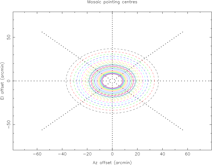
The pattern of pointings is shown in Figure broadmap.
The pointing pattern used to map the shape of the beam for the new 16cm
receivers out past the primary lobe. Each black dot is the location of a pointing
centre, while the solid circles represent the expected primary beam FWHM at
various frequencies (being plotted are 1268, 1396, 1524, 1652, 1780, 1908,
2036, 2164, 2292, 2420, 2548, 2676, 2804 and 2932 MHz). Each dashed circle has twice
the radius of the solid circle with the same colour.
Fine polarisation purity measurements
The second set of measurements was made over three epochs: September 2 and 9, 2011, and
November 3 2011. By this time, each of the ATCA antennas had an upgraded 16cm receiver.
The purpose of these observations was to determine how the polarisation measured for
a source with known polarisation varied dependent on its position in the primary beam.
For these observations, the central frequency was set to be 2100 MHz.
The measurements were conducted as for the broad beamshape measurements, with the
reference antenna being CA06. The source used for these measurements was PKS B1934-638,
as it is known to have zero linear polarisation (Stokes Q and U) and very small
circular polarisation (Stokes V).
The azimuth and zenith offsets were designed to make a radial grid of pointings, using
a similar radial cut procedure. The cuts were made at 22.5° intervals, to ensure
finer sampling but continue to assess the effect of the feed legs at 45° angles.
Along each cut, the radial distance between each offset point was set at 3 arcminutes.
Thirteen pointings were made along each radial cut, corresponding to a maximum distance
of 39 arcminutes.
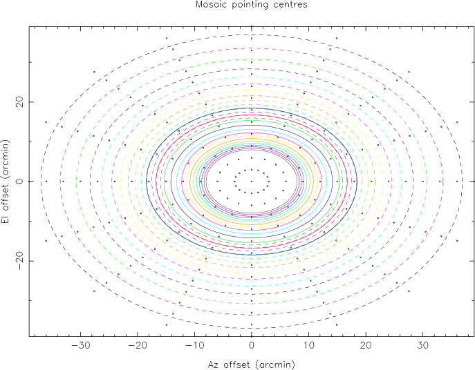
The pattern of pointings is shown in Figure finemap.
The pointing pattern used to assess the off-axis polarisation properties for the new 16cm
receivers. Each black dot is the location of a pointing
centre, while the solid circles represent the expected primary beam FWHM at
various frequencies (being plotted are 1268, 1396, 1524, 1652, 1780, 1908,
2036, 2164, 2292, 2420, 2548, 2676, 2804 and 2932 MHz). Each dashed circle has twice
the radius of the solid circle with the same colour.
The integration time on each pointing was set to be 24 seconds (using a CABB cycle time
of 6 seconds). Sensitivity was key in this experiment because the RMS noise level might
perhaps be the limiting factor in assessing the off-axis polarisation purity; the goal
is to measure zero flux density from each pointing.
Leakage determination measurements
The linear polarisation of the ATCA primary flux calibrator PKS B1934-638 is known to be
very small (and assumed to be zero) at low frequencies. It should therefore be possible
to calculate the cross-polarisation leakage terms for each antenna based only on an
observation of this calibrator. The normal procedure for determining leakages from a
calibrator with unknown (but assumed constant) polarisation properties, is to make a set
of observations across a sufficiently large range of parallactic angles. This is generally
possible for a full synthesis observation where phase-referencing is undertaken, but may
be a problem for short observations, such as for Target-of-Opportunity (ToO) observations.
The goal of these observations was to determine if a single observation of 1934-638 would
provide the same leakage solution as the conventional method.
To test this, we observed a number of sources over 12 hours on each of two epochs:
November 3 and 25, 2011. Each source could be used to derive a leakage solution to compare
to that obtained from 1934-638.
Data Reduction
The following sections describe in some detail the data reduction process used for each
of the different datasets. The Miriad tasks used for the reduction, and the reasons for
their use will be described.
Broad beamshape measurements
RPFITS files
2010-08-25_2207.C999
2010-08-25_2225.C999
Procedure
Load the data in the normal way.
atlod ifsel=1 options=birdie,xycorr,noauto
Since the data coming in to both
CABB IFs is identical (apart from conversion and digitiser noise and subsequent correlation),
we choose only to analyse the first IF.
Flag the unused antenna.
uvflag flagval=flag "select=ant(1,5)"
Flag the setup data.
uvflag flagval=flag "select=time(22:00,22:26)"
Flag some edge channels that are affected by the bandpass rolloff.
uvflag flagval=flag edge=40
Split into individual pointings with uvsplit.
The first pointing of each radial observation puts 0823 at the beam centre. To
correctly calibrate these pointings, we change their name to 0823-500.
uvputhd hdvar=source varval=0823-500
We then put all these pointings into a single dataset with uvcat,
taking care that each scan is added in the correct time order.
Do an initial round of automatic flagging before calibration, which will get rid of the
biggest and most obvious RFI.
We now recalibrate, using 16 frequency bins in gpcal.
mfcal
gpcal interval=0.1 nfbin=16 options=xyvary
For each off-source pointing, we copy the calibration from 0823-500 using
gpcopy, and then use threshold flagging to remove
the RFI.
We prepare the off-source pointings to be split into multiple frequency
chunks by applying the calibration solutions with uvaver.
Each off-source pointing is split into 16 128 MHz frequency chunks.
uvsplit maxwidth=0.128
We measure the beam response in two ways. The voltage response is measured between each
off-source antenna and the on-source reference (CA02 in this case). The power response
is measured on the baselines formed by the off-source antenna (CA03, CA04 and CA06).
We measure the flux observed by each of six baselines per pointing: 2-3, 2-4, 2-6,
3-4, 3-6 and 4-6.
The uvfmeas task is used to make the measurements
of flux density because it can make a fit to the spectral data. This allows a consistent
measurement of the flux density at the same frequency each time. Because each
pointing is flagged separately, it is possible for the average flux measurement of any
particular pointing to be at an arbitrary effective frequency. Making a fit and evaluating
it for a consistent frequency should alleviate this problem.
Fine polarisation purity measurements
RPFITS files
2011-09-02_1516.C2511
2011-09-02_1721.C2511
2011-09-02_1826.C2511
2011-09-09_1406.C2511
2011-11-03_0442.C2511
2011-11-03_0646.C2511
2011-11-03_0849.C2511
2011-11-03_1052.C2511
2011-11-03_1255.C2511
Procedure
The reduction for each day's data is made in the same way as for the broad beamshape
data. The primary difference is that the mosaic order is different for these observations,
and the on-source location is visited only once per mosaic iteration which covers all the
offset pointings. We still take the "phase" source, rename it as 1934-638 using
uvputhd and add it to a combined 1934-638 dataset which we use
for calibration.
The beam response is measured as before, although each the reference antenna changes from
CA06 on 2011-09-02 and 2011-09-09, to CA02 on 2011-11-03.
The reference antenna stayed on source, and
all the other antennas were available each day. To get the voltage responses,
we measure the Stokes I flux densities observed by each of five baselines with the reference antenna.
We also the Stokes I, Q, U and V flux densities observed by the other ten baselines.
For the Stokes I measurements we use the
scalar average option in uvfmeas, but for the measurements of other
Stokes parameters, we use vector averaging as those flux densities can be negative.
Results
Broad beamshape measurements
Pointing corrections
The first task is to determine the pointing errors for each antenna during the experiment.
We do this by roughly following the procedure described in the first "Measurements of the
ATCA primary beam" memo by M.H. Wieringa and M.J. Kesteven.
We take the beam voltage response measurements made at each offset point, for each antenna, and
scale it to the most recent on-source flux density. In this way, we now deal with ratios.
A Gaussian curve following the equation
\[A(r) = ae^{-4\log(2)((r - c)/fwhm)^2},\]
(where \( a \) is the peak height scaling of the curve,
\( r \) is the radial distance from the centre position,
\( c \) is the location of that centre (which may not be zero), \( fwhm \) is
the FWHM of the Gaussian function, and \( \log \) represents a natural logarithm)
is fitted to measurements with a ratio \( \geq 0.3 \), for each of the radial spokes.
The median of the eight spokes' FWHM is calculated, and kept fixed while fitting another
Gaussian for each of the eight spokes, this time in order to determine the peak centre and
height. We assume here that the beam is symmetrical (at least out to the 30% level) in order
to calculate the pointing offsets.
We do this fitting using the frequency chunk centred on 2548 MHz, which we think is the
most sensitive area of the bandwidth. Each spoke's pointing offsets are determined and
corrected separately. This is justified due to the time between the observations of each
spoke (around 30 minutes), and the fact that the telescope was performing this experiment
as 0823-500 was transiting.
The pointing errors found in this way ranged between 0.5″ and 38″, and were
smallest on CA06. The average pointing error was \( \sim \) 12″.
After these pointing corrections are made, the appropriate scaling of the curves
is calculated by fitting another fixed-width Gaussian, but this time forcing the centre
to be at 0. These scaling corrections are determined per spoke and per frequency,
since the width of the Gaussian differs with frequency. The average peak scaling over
all the frequencies and spokes is 1.01.
The pointing corrections are applied to the power response measurements by taking the
average correction based on each individual antenna's correction.
Gaussian fitting
With the pointing-corrected data, we fit a Gaussian curve following the form
\[A(x) = e^{-4\log(2)(x/fwhm)^2},\]
where \( x \) is the normalised distance from the centre, and is simply defined as
the distance in arcminutes multiplied by the frequency in GHz, such that the point (for example)
\( x = 35 \) corresponds roughly to the 20% power level at all frequencies. Note that this
equation has no variables for the centre position or the curve scaling height, as these are
set to be 0 and 1 respectively.
The Gaussian fit is made to points out to \( x = 35 \) arcmin GHz.
The fit coefficient \( fwhm \) - the full-width at half-maximum of the Gaussian curve -
is listed in Table gaussian_fwhm.
Frequency
\( fwhm \)
[MHz]
[arcmin GHz]
1268
46.53
1396
47.58
1524
48.91
1652
49.35
1780
50.05
1908
50.70
2036
51.22
2164
50.61
2292
50.01
2420
49.66
2548
49.61
2676
49.48
2804
48.81
2932
48.31
Gaussian full-width half maxima as fitted to data from all angles at each frequency, assuming
a curve centred at \( x = 0 \), with a peak height of 1.
The Gaussian fits made by Wieringa and Kesteven in their memo covered the same range of
\( x \), and are very similar to the fits we make here. In their 20cm band (centred
on 1420 MHz) they fit a \( fwhm \) of 47.9 arcmin GHz, while in their 13cm band
(centred on 2358 MHz) it is 49.7 arcmin GHz.
Our fits here show that the \( fwhm \) changes in an orderly fashion over the frequency range,
getting larger from low frequencies and reaching a maximum in the band centred on 2036 MHz, before
getting smaller as the frequency increases. It would be interesting to see if these numbers
are affected, or could be tuned by varying the subreflector focus position. The fits to the data
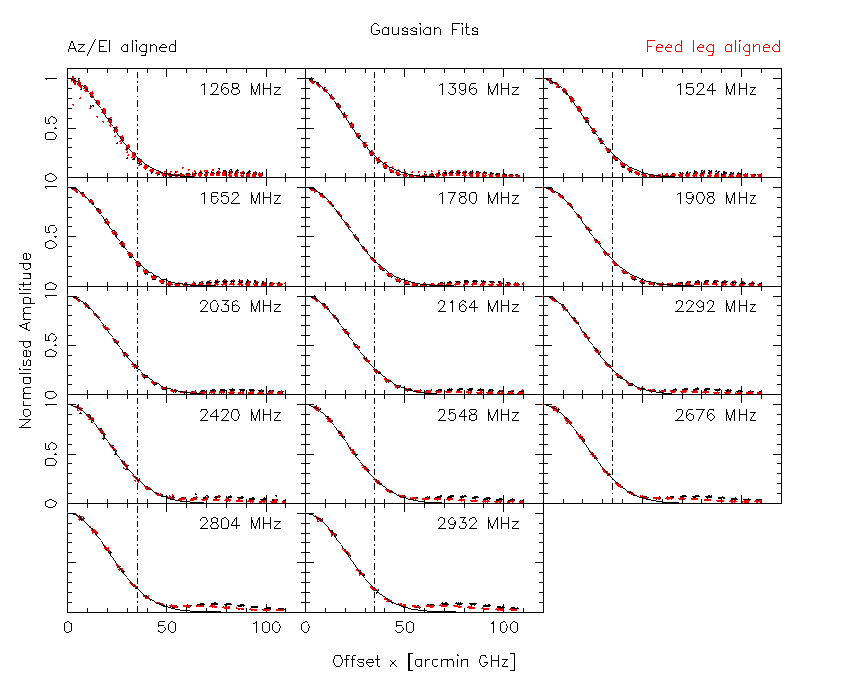
are shown in Figure gaussian_fits.
The Gaussian fits to the data. Each panel represents data taken at the frequency
shown in its top-right. The black points indicate measurements along angles that align with
the azimuth or elevation axes, while the red points are along angles that intersect the feed
support legs. The solid black line is the Gaussian fit to the panel's data, while the vertical
dot-dashed line represents \( x = 35 \), the usability limit of the fit.
We can assess how well the fits describe the data by simply determining the absolute sum
of the differences between the data with \( x \leq 35 \) and the Gaussian fit. This does not
necessarily tell us anything useful in an absolute sense, but does allow us to compare our new fits
with those made by Wieringa and Kesteven.
An examination of the fit quality in this way reveals that for the sets with central frequencies
less than 2164 MHz, each set is best described by its own fit, and the same is true for the sets
at 2548, 2804 and 2932 MHz. For the other frequencies, the situation is as follows.
At 2164 MHz, the best fit is from the 1908 MHz data, although there is only a 0.09% difference
between the fit quality scores.
At 2292 MHz, the best fit is from the 1780 MHz data, although there is only a 0.02% difference
between the fit quality scores.
At 2420 MHz, the best fit is from the 13cm Wieringa and Kesteven data, although there is only
a 0.02% difference between the fit quality scores.
At 2676 MHz, the best fit is from the 1652 MHz data, although there is only a 0.05% difference
between the fit quality scores.
With these small differences in mind, we will use each data's own fit to describe it.
PBCOR fitting
The AIPS task PBCOR uses primary beam fits that have the form
Fits to this equation are made using data out to \( x = 50 \), which represents data out to about
the 3% level of the beam. The fits were made via a weighted linear least-squares method, where
the weights were specified to be inversely proportional to the square of the distance from the
centre. This was done because an unweighted fit more closely matched the outer parts of the beam than
the inner parts. The PBCOR fit coefficients are shown in Table
pbcor_coefficients,
and the fits are shown graphically in Figure pbcor_fits.
Frequency [MHz]
\( a_{1} \)
\( a_{2} \)
\( a_{3} \)
\( a_{4} \)
1268
+2.27e-03
-2.21e-06
+1.75e-09
+6.68e-13
1396
+1.46e-03
+2.29e-06
-4.15e-09
+2.54e-12
1524
+1.50e-03
+2.45e-07
-6.93e-10
+1.05e-12
1652
+1.41e-03
+2.15e-07
-3.77e-10
+8.16e-13
1780
+1.40e-03
-4.75e-08
+6.82e-11
+5.27e-13
1908
+1.22e-03
+5.62e-07
-4.80e-10
+5.99e-13
2036
+1.24e-03
-1.31e-07
+6.85e-10
+7.82e-14
2164
+1.21e-03
-7.08e-08
+8.89e-10
-3.52e-14
2292
+1.26e-03
-3.49e-08
+7.74e-10
+3.95e-14
2420
+1.20e-03
+1.43e-07
+8.18e-10
-4.56e-14
2548
+1.24e-03
-8.58e-08
+1.13e-09
-1.43e-13
2676
+1.24e-03
-3.30e-08
+1.09e-09
-1.42e-13
2804
+1.22e-03
+2.19e-07
+9.06e-10
-8.53e-14
2932
+1.39e-03
-3.51e-07
+1.53e-09
-2.39e-13
20cm
+8.99e-04
+2.15e-06
-2.23e-09
+1.56e-12
13cm
+1.02e-03
+9.48e-07
-3.68e-10
+4.88e-13
The PBCOR fit coefficients, as fitted to data from all angles at each frequency. The
Wieringa and Kesteven fits are shown as band names rather than as frequency.
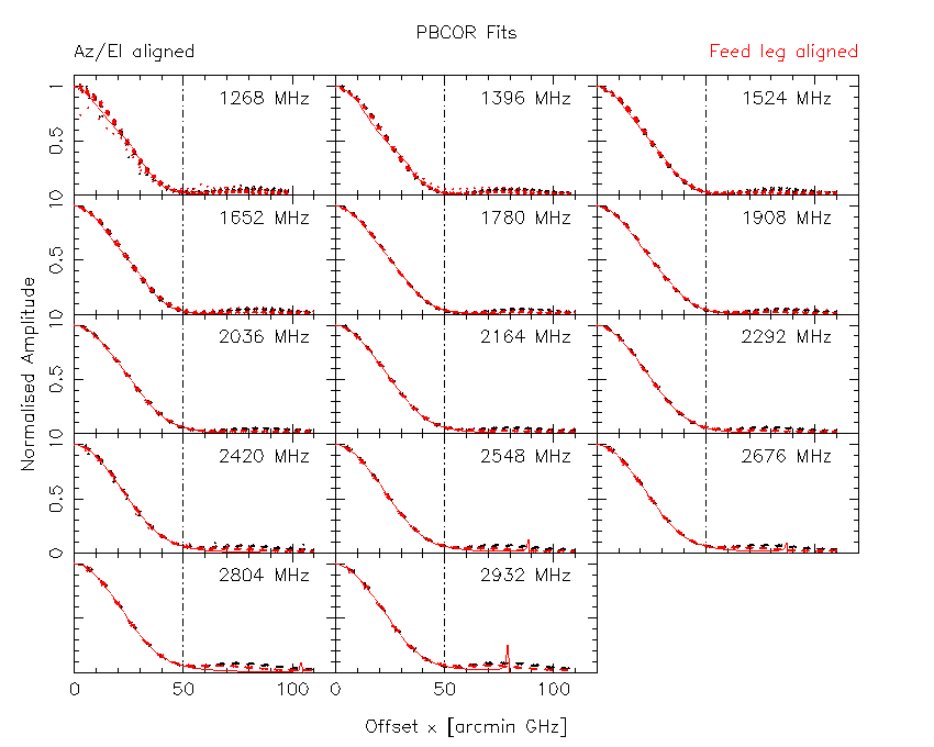
The PBCOR fits to the data. Each panel represents data taken at the frequency
shown in its top-right. The black points indicate measurements along angles that align with
the azimuth or elevation axes, while the red points are along angles that intersect the feed
support legs. The solid red line is the PBCOR fit to the panel's data, while the vertical
dot-dashed line represents \( x = 50 \), the usability limit of the fit.
An examination of the fit quality scores tells us that the data at 1652, 2036, 2164, 2292,
2420, 2676, 2804 and 2932 MHz are all best described by their own fits. For the other
frequencies:
The data at 1268, 1396 and 1524 MHz are all better described by the 20cm fit of
Wieringa and Kesteven, by 13.7%, 30.7% and 5.3% respectively.
The data at 1780 MHz is better described by the 13cm fit of Wieringa and Kesteven,
by 17.9%.
The data at 1908 MHz is better described by the fit made at 2164 MHz, by 4.6%.
The data at 2548 MHz is better described by the fit made at 2676 MHz, by 0.6%.
The reason for the poor fits at these frequencies is not yet known.
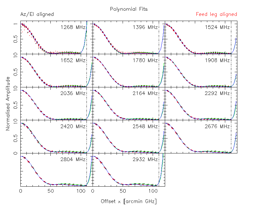
Polynomial fitting
A higher order fit can be made to the data in order to characterise the outer portions
of the beam power response, past the first null and into the first sidelobe. It is clear
from Figures gaussian_fits and pbcor_fits
that the shape of the beam past the first null is dependent on the angle with respect to the feed legs,
so we make two separate fits in this regime: one for the shape aligned with the azimuth and elevation
directions, and another aligned with the feed support legs.
where only the even powers of \( x \) are used, since these are the terms present in
the theoretical beam response \( J_{1}(r)/r \). These fits were made via a weighted linear
least-squares method, where the weights were inversely proportional to the square of
the measurement uncertainty of the flux densities. The polynomial fit coefficients are shown
in Table polynomial_coefficients and the fits are shown
graphically in Figure polynomial_fits. The fits use data out to
\( x = 110 \).
Frequency [MHz]
dir.
\( a_{1} \)
\( a_{2} \)
\( a_{3} \)
\( a_{4} \)
\( a_{5} \)
\( a_{6} \)
1268
+
-1.154e-03
+5.351e-07
-1.265e-10
+1.634e-14
-1.099e-18
+3.009e-23
1268
x
-1.163e-03
+5.481e-07
-1.317e-10
+1.718e-14
-1.159e-18
+3.173e-23
1396
+
-1.092e-03
+4.660e-07
-9.875e-11
+1.119e-14
-6.504e-19
+1.522e-23
1396
x
-1.099e-03
+4.769e-07
-1.032e-10
+1.187e-14
-6.950e-19
+1.628e-23
1524
+
-1.048e-03
+4.305e-07
-8.824e-11
+9.684e-15
-5.446e-19
+1.232e-23
1524
x
-1.054e-03
+4.407e-07
-9.229e-11
+1.030e-14
-5.843e-19
+1.327e-23
1652
+
-1.033e-03
+4.221e-07
-8.692e-11
+9.679e-15
-5.571e-19
+1.298e-23
1652
x
-1.043e-03
+4.343e-07
-9.131e-11
+1.029e-14
-5.939e-19
+1.376e-23
1780
+
-1.003e-03
+4.016e-07
-8.170e-11
+9.046e-15
-5.199e-19
+1.213e-23
1780
x
-1.013e-03
+4.135e-07
-8.589e-11
+9.612e-15
-5.521e-19
+1.276e-23
1908
+
-9.794e-04
+3.831e-07
-7.562e-11
+8.067e-15
-4.440e-19
+9.882e-24
1908
x
-9.909e-04
+3.967e-07
-8.062e-11
+8.807e-15
-4.926e-19
+1.107e-23
2036
+
-9.692e-04
+3.848e-07
-7.809e-11
+8.621e-15
-4.927e-19
+1.140e-23
2036
x
-9.847e-04
+4.023e-07
-8.461e-11
+9.636e-15
-5.637e-19
+1.326e-23
2164
+
-9.919e-04
+4.028e-07
-8.251e-11
+9.077e-15
-5.122e-19
+1.163e-23
2164
x
-1.008e-03
+4.204e-07
-8.903e-11
+1.008e-14
-5.812e-19
+1.339e-23
2292
+
-1.007e-03
+4.131e-07
-8.480e-11
+9.305e-15
-5.220e-19
+1.176e-23
2292
x
-1.028e-03
+4.353e-07
-9.309e-11
+1.060e-14
-6.122e-19
+1.411e-23
2420
+
-1.016e-03
+4.235e-07
-8.817e-11
+9.772e-15
-5.521e-19
+1.251e-23
2420
x
-1.035e-03
+4.432e-07
-9.541e-11
+1.090e-14
-6.305e-19
+1.453e-23
2548
+
-1.033e-03
+4.375e-07
-9.223e-11
+1.033e-14
-5.885e-19
+1.343e-23
2548
x
-1.050e-03
+4.565e-07
-9.954e-11
+1.149e-14
-6.708e-19
+1.559e-23
2676
+
-1.035e-03
+4.395e-07
-9.269e-11
+1.038e-14
-5.919e-19
+1.353e-23
2676
x
-1.050e-03
+4.568e-07
-9.927e-11
+1.140e-14
-6.609e-19
+1.525e-23
2804
+
-1.064e-03
+4.622e-07
-9.913e-11
+1.125e-14
-6.502e-19
+1.505e-23
2804
x
-1.079e-03
+4.827e-07
-1.074e-10
+1.259e-14
-7.454e-19
+1.758e-23
2932
+
-1.081e-03
+4.769e-07
-1.045e-10
+1.222e-14
-7.325e-19
+1.768e-23
2932
x
-1.097e-03
+4.980e-07
-1.128e-10
+1.355e-14
-8.259e-19
+2.012e-23
20cm
+
-1.078e-03
+4.618e-07
-1.011e-10
+1.207e-14
-7.513e-19
+1.908e-23
20cm
x
-1.049e-03
+4.238e-07
-8.473e-11
+9.073e-15
-5.004e-19
+1.118e-23
13cm
+
-1.032e-03
+4.340e-07
-9.337e-11
+1.088e-14
-6.553e-19
+1.598e-23
13cm
x
-9.942e-04
+3.932e-07
-7.772e-11
+8.239e-15
-4.492e-19
+9.899e-24
The polynomial fit coefficients, as fitted to data at angles aligned with the
azimuth/elevation axes (represented as the + direction) and at angles aligned
with the feed support legs (represented as the x direction). The Wieringa and
Kesteven fits are shown as band names rather than as frequency. Note also that
the direction convention used here is opposite to that used by Wieringa and
Kesteven, but is normalised to our convention for this table.
The polynomial fits to the data. Each panel represents data taken at the frequency
shown in its top-right. The black points indicate measurements along angles that align
with the azimuth or elevation axes, while the red points are along angles that
intersect the feed support legs. The solid green line is the polynomial fit to the
panel's data along the azimuth/elevation axes, while the solid blue line is the fit
along the feed support leg axes. The vertical dot-dashed line represents \( x = 110 \),
the usability limit of the fits.
We find here a clear and unsurprising trend that the data from each frequency and angle set is
characterised best by its own fit.
Fine polarisation purity measurements
Pointing corrections
The pointing corrections are determined in the same way as for the broad beamshape measurements.
Each day's corrections were determined separately and without using any information from other days,
or from the broad beamshape experiment. The pointing errors had roughly the same range each day as for
the broad beamshape experiment.
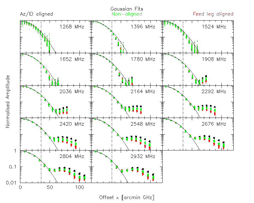
Comparison with broad beamshape fits
To check that the reduction and measurements have been successful, we compare the fits made to the
broad beamshape experiment data to the data from this experiment. It should be noted that the plots
shown in Figures gaussian_fits_comparison,
pbcor_fits_comparison and polynomial_fits_comparison
do not include data from the angles 180° and 202.5° in the 2011-11-03 epoch, since that data was
corrupted.
We further split the data into another set of angles, that fit between the Az/El-aligned axis and the
feed leg-aligned axis. We call these the "Non-aligned" angles.
The Gaussian fits to the broad beamshape data are plotted on top of the data taken
as part of the fine polarisation purity experiment. Each panel represents data taken at the frequency
shown in its top-right. The black points indicate measurements along angles that align
with the azimuth or elevation axes, the red points are along angles that
intersect the feed support legs, and the green points are along other non-aligned angles.
The solid black line is the Gaussian fit to the
panel's data, while the vertical dot-dashed line represents \( x = 35 \),
the usability limit of the fits.
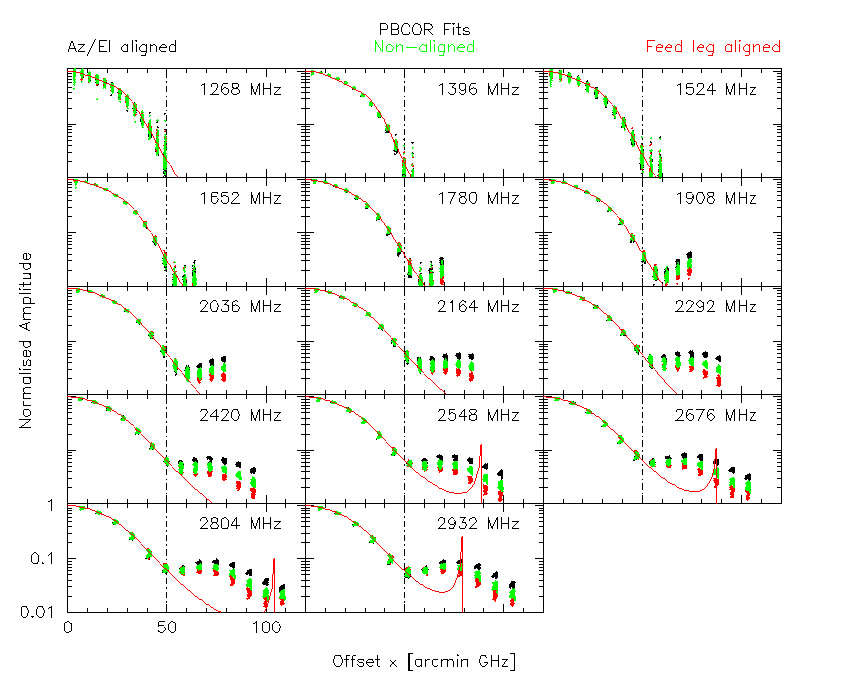
The PBCOR fits to the broad beamshape data are plotted on top of the data taken
as part of the fine polarisation purity experiment. Each panel represents data taken at the frequency
shown in its top-right. The black points indicate measurements along angles that align
with the azimuth or elevation axes, the red points are along angles that
intersect the feed support legs, and the green points are along other non-aligned angles.
The solid red line is the Gaussian fit to the
panel's data, while the vertical dot-dashed line represents \( x = 50 \),
the usability limit of the fits.
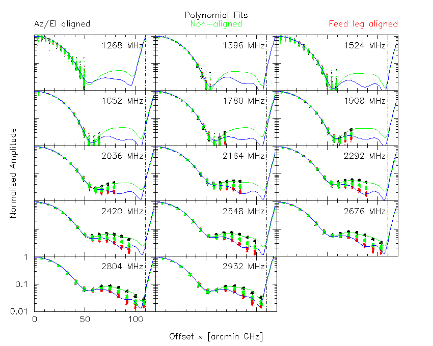
The polynomial fits to the broad beamshape data are plotted on top of the data taken
as part of the fine polarisation purity experiment. Each panel represents data taken at the frequency
shown in its top-right. The black points indicate measurements along angles that align
with the azimuth or elevation axes, the red points are along angles that
intersect the feed support legs, and the green points are along other non-aligned angles.
The solid green line is the polynomial fit to the
panel's data along the azimuth/elevation axes, while the solid blue line is the fit
along the feed support leg axes. The vertical dot-dashed line represents \( x = 110 \),
the usability limit of the fits.
The comparison between this data and the beam fits is excellent, so we can be confident that our
data is of high quality.
It is interesting to see that the non-aligned angles at large \( x \) values have beam ratios that
lie between the feed-leg aligned ratios and the Az/El-aligned ratios. This may further complicate the
primary beam correction when out at such large distances from the beam centre.