ATCA Calibrator Database v3

Documentation

Introduction

Version 3 of the ATCA calibrator database represents a number of major improvements, meant to improve the accuracy and reliability of the data it presents. This documentation describes:

the measurement process that produces the information contained in the calibrator database,
how to use the web interface to find the information you require,
how to interpret the numbers and graphs presented by the web interface.

This documentation was last updated on 2014-Jan-21.

The Measurement Process

Loading the data

Loading the data is done manually, to screen out RPFITS files that have calibration data in them (data during a dcal, pcal or acal for example). If these data are mixed in with useful data then the calibration data is manually flagged as bad.

The atlod step is done the same way for every band. For CABB data:


	      atlod "in=*.C007" options=birdie,rfiflag,noauto,xycorr,opcorr nopcorr=32 out=c007.uv

This command flags out all the frequency ranges that are commonly affected by bad RFI, discards any autocorrelation data, corrects for phase offsets between the X and Y polarisations on each antenna and compensates for atmospheric opacity in 32 discrete bins across each 2 GHz band. We do the opacity correction on such a fine scale because in certain areas of the band (at high frequencies, and near water lines for example), the opacity can change very quickly as a function of frequency. Correcting opacity in this way will make it less likely that our bandpasses will have curvature caused by atmospheric effects later in our reduction.

For pre-CABB data:


	      atlod "in=*.C007" options=birdie,reweight,noauto,xycorr,nocacal,opcorr \

	        nopcorr=2 out=c007.uv

This makes the opacity correction happen at the same resolution (64 MHz) as for the CABB data, and does some pre-CABB correlator reweighting to get rid of Gibbs ringing.

If the observations in this epoch are made in the 3mm band, we now need to interpolate the system temperatures derived at each paddle scan; we do this with atfix:


	      atfix vis=c007.uv out=c007a.uv tsyscal=interpolate

We now split the data into sources, and deal with each band that was observed separately, by using directories that are named for the band. Except at 16cm, this means that there will be two separate frequencies, usually separated by 2 GHz or more, in each directory.

Bandpass and flux calibration

There are two distinctly different schemes for bandpass calibration. In the 16cm and 4cm bands, where the ATCA flux calibrator 1934-638 is bright enough to act as the bandpass calibrator, bandpass calibration is done simply by running mfcal on its dataset at each band frequency. For example, if we were reducing data at 16cm:


	      mfcal vis=1934-638.2100 interval=0.1

We use an interval of 0.1 minutes for the time-dependent gain solution so that short-term variations do not get transferred into the bandpass solution.

We then do further calibration with gpcal:


	      gpcal vis=1934-638.2100 interval=0.1 options=xyvary nfbin=2

We now do some automatic flagging using the AOFlagger algorithm in pgflag:


	      pgflag vis=1934-638.2100 stokes=xx,yy command=<b

	      pgflag vis=1934-638.2100 stokes=yy,xx command=<b

With flagging done, we delete all the calibration tables and redo the exact same calibration commands as before, after which we consider the flux and bandpass calibration to be done.

In higher frequency bands where the flux calibrator cannot be used as the bandpass calibrator, either because it is too faint (as in the case of 1934-638 in the mm bands) or too large (as for Uranus), we need to use a more intricate calibration scheme.

We begin by choosing a very bright calibrator from the list of those observed during the epoch. Usually this is one of the usual array setup calibrators, like 0537-441, 1253-055 or 1921-293 for example. We do the initial bandpass calibration as before:


	      mfcal vis=1921-293.17000 interval=0.1

	      mfcal vis=1921-293.19000 interval=0.1

The problem that arises here though is that because there is no definitive apriori information about the brightness and spectral behaviour of the bandpass calibrator, the bandpass solution will be wrong. Miriad assumes that the bandpass calibrator has a flat-spectrum (the same flux density in each frequency channel), which is likely to be incorrect for almost all calibrators.

Let's look at just how wrong this is. We do this using the new Miriad task written especially for the v3 calibrator database, uvfmeas. We can look at the spectral behaviour of the bandpass calibrator over the observed frequency range.


	      uvfmeas vis=1921-293.1[79]000 stokes=i order=1 options=plotvec,log device=/xs

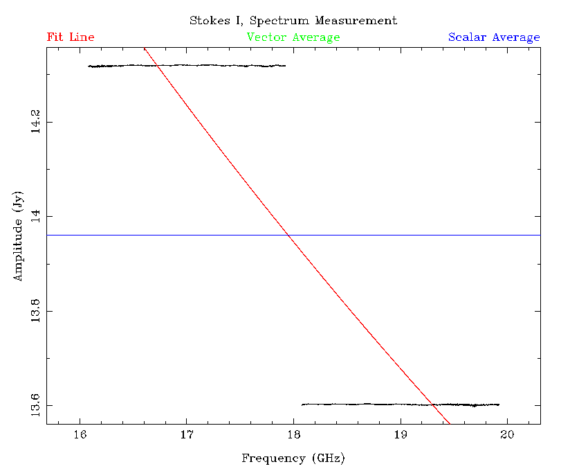
The bandpass calibration seems to have worked pretty well, since the flux density in each band is constant over frequency, with only small deviations. But the source is unlikely to be actually flat-spectrum, as evidenced by the observation that the flux density in each band is significantly different.

We thus have to determine the bandpass calibrator's spectral behaviour and flux density. To do this we copy the the solution we have just made to the flux calibrator to determine how wrong it is. But the way this is done is different depending on whether the flux calibrator is 1934-638 or Uranus. We deal with the case of 1934-638 first.

The first step here is to do a further calibration with gpcal:


	      gpcal vis=1921-293.17000 interval=0.1 options=xyvary nfbin=2

	      gpcal vis=1921-293.19000 interval=0.1 options=xyvary nfbin=2

And then copy these solutions to 1934-638:


	      gpcopy vis=1921-293.17000 out=1934-638.17000

	      gpcopy vis=1921-293.19000 out=1934-638.19000

And then calibrate 1934-638 with gpcal:


	      gpcal vis=1934-638.17000 interval=0.1 options=xyvary nfbin=2

	      gpcal vis=1934-638.19000 interval=0.1 options=xyvary nfbin=2

It is at this point that automatic flagging may be done on both the bandpass and flux calibrators, but in most cases very little flagging is required, and this step can usually be omitted.

Because we have solved for time-varying gains in two bins across the band, gpcal can deal with both absolute scaling of flux density, and with a slope correction due to the error built into the bandpass solution:


	      gpboot vis=1921-293.17000 cal=1934-638.17000

	      gpboot vis=1921-293.19000 cal=1934-638.19000

At this point we use uvfmeas to examine the spectrum of the bandpass calibrator in the same way as before.

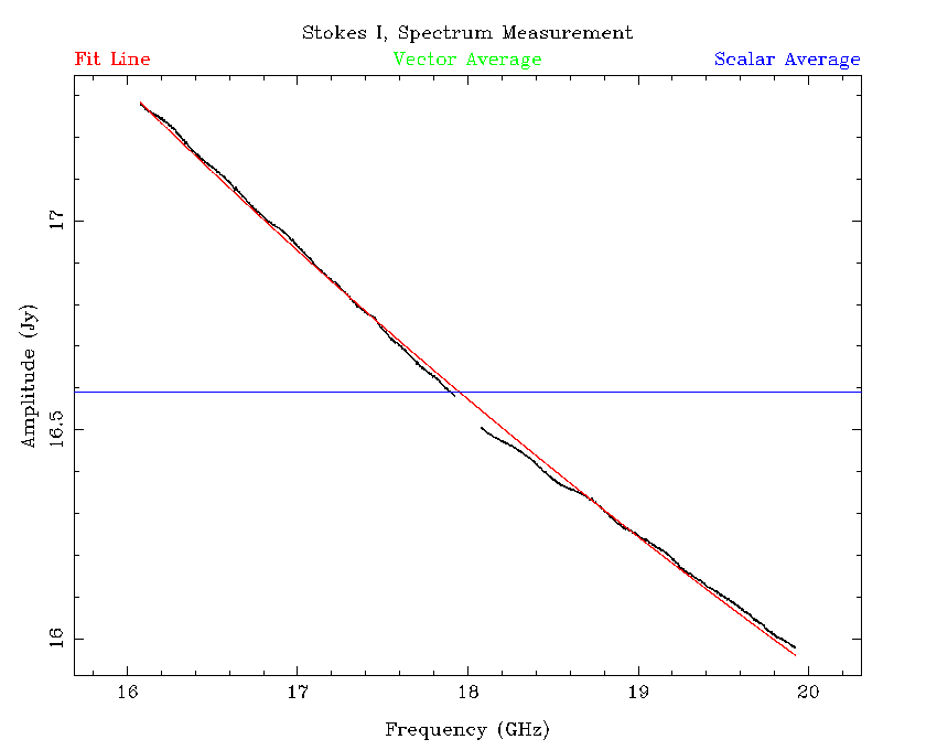
Already this looks like a very large improvement, as the bands almost join smoothly to each other; recall that the reduction of the bands have been completely independent. However the agreement between the bands is not perfect, and the bandpass function itself is still incorrect.

On the plot above that uvfmeas generated, there is a red line; this is the least-squares linear fit to $\log {\rm S} / \log\nu$. On this occasion, the line of best fit is

$\log({\rm S} / 1 {\rm\,Jy}) = 1.685 - 0.3711\log(\nu / 1 {\rm\,GHz}),$

and there is an RMS scatter of 13.85 mJy of the measured flux densities around this fit line. This would suggest that this fit is accurate to 1%, although there could still be uncertainty in the absolute flux scaling. Investigations of absolute calibration accuracy was done with simulations, and in that case it was possible to get better than 1% accuracy on the bandpass calibrator's flux density using this method, even if the fit made to each band separately could be in error by as much as 10%.

To correct the bandpass function we go back to mfcal and input the now known flux density model for the bandpass calibrator:


	      mfcal vis=1921-293.17000 interval=0.1 flux=16.9286,17.0,-0.3711

	      mfcal vis=1921-293.19000 interval=0.1 flux=16.9286,17.0,-0.3711

Here, the flux specification is taken directly from the output of uvfmeas with the mfflux option given.

We can now redo the flux calibration with 1934-638 as before. After this, the best fit changes to:

$\log({\rm S} / 1 {\rm\,Jy}) = 1.685 - 0.3713\log(\nu / 1 {\rm\,GHz}),$

and the RMS scatter is decreased to 13.33 mJy. This of course is not a large improvement, but simulations indicate that doing this significantly improves the accuracy of flux density measurements for the other sources that the bandpass calibration is applied to.

If the flux calibrator is Uranus, then the procedure is slightly different. We start the procedure in a similar way, by doing the mfcal and gpcal steps on the bandpass calibrator:


	      mfcal vis=1921-293.33000 interval=0.1

	      mfcal vis=1921-293.35000 interval=0.1

	      gpcal vis=1921-293.33000 interval=0.1 options=xyvary

	      gpcal vis=1921-293.35000 interval=0.1 options=xyvary

Then we copy the gain and bandpass solutions to the flux calibrator:


	      gpcopy vis=1921-293.33000 out=uranus.33000

	      gpcopy vis=1921-293.35000 out=uranus.35000

And use mfboot to correct the bandpass and flux scale:


	      mfboot vis=1921-293.33000,uranus.33000 device=/xs "select=source(uranus)"

	      mfboot vis=1921-293.35000,uranus.35000 device=/xs "select=source(uranus)"

From this point, we measure the best fit flux density model with uvfmeas as before, and redo the entire calibration routine again while specifying the measured fit in the mfcal stage.

At this point we consider that the bandpass and flux calibrators have the correct bandpass solution, and are on the correct absolute flux scale. We can now proceed to calibrate the rest of the sources.

Source calibration

The other sources observed during an epoch can easily be calibrated simply by copying the solutions from the bandpass calibrator, running gpcal, doing some automatic flagging and repeating the process. This, for the most part, is independent of the band that we are calibrating. To keep them on the same flux scale, we run gpboot with the bandpass calibrator as the reference after the gpcal stage. As an example, for a source in the 4cm band, the calibration method might look like the following:


	      gpcopy vis=1934-638.5500 out=0420-014.5500

	      gpcopy vis=1934-638.9000 out=0420-014.9000

	      gpcal vis=0420-014.5500 interval=0.l options=xyvary,qusolve,nopol nfbin=2

	      gpcal vis=0420-014.9000 interval=0.l options=xyvary,qusolve,nopol nfbin=2

	      pgflag vis=0420-014.5500 stokes=xx,yy "command=<b"

	      pgflag vis=0420-014.5500 stokes=yy,xx "command=<b"

	      gpcopy vis=1934-638.5500 out=0420-014.5500

	      gpcopy vis=1934-638.9000 out=0420-014.9000

	      gpcal vis=0420-014.5500 interval=0.l options=xyvary,qusolve,nopol nfbin=2

	      gpcal vis=0420-014.9000 interval=0.l options=xyvary,qusolve,nopol nfbin=2

	      gpboot vis=0420-014.5500 cal=1934-638.5500

	      gpboot vis=0420-014.9000 cal=1934-638.9000

We keep using nfbin=2 so that gpboot can also correct for any slightly frequency-dependent effects that may be present in the data.

This calibration method is quite robust, and rarely needs manual intervention, due to the way we do the measurement of flux densities. But there is a weakness that will need to be solved at some future point: polarisation calibration is not guaranteed to be very good here. The problem is that during C007 observations, a source might be observed only for a few minutes in one hit, and this includes both the bandpass and flux calibrators as well. Since this is not sufficient parallactic angle coverage from which to reliably determine leakages, the polarisation is not well determined. At low frequencies, where 1934-638 is known to have very small linear polarisations, leakages determined from it are generally not too bad, and polarisation calibration of the other sources is also reasonable so long as we specify options=qusolve,nopol during the gpcal stage (this means that we accept the leakages determined from 1934-638). At higher frequencies, there is no real expectation that polarisations will be calibrated correctly.

The calibrator database does not currently measure polarisations for each source because of this known weakness, but work is underway to determine some polarisation calibrators at all frequencies so this can be resolved in the future.

Measuring the flux density models

After the calibration process has been completed, we use uvfmeas to determine best fit flux density models. For example, in the 4cm band, here is the procedure for measuring the flux density model for the source 2244-372 in the 2012-Apr-22 C007 epoch:


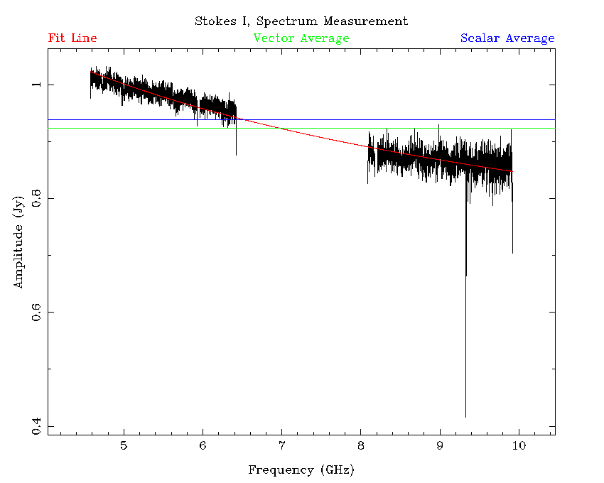
	      uvfmeas vis=2244-372.5500,2244-372.9000 options=plotvec,log order=1 \

	      device=/xs stokes=i

The output from this command is:

Source: 2244-372
Stokes I
Vector Average Amplitude:   9.237E-01         Phase:  -1.426E-06
             Uncertainty:   7.311E-01
Scalar Average Amplitude:   9.379E-01   Uncertainty:   7.211E-01
Vector Average Fit Coefficients:
 log S =   1.705E-01
       +  -2.432E-01 x (log f)^ 1
Scatter around fit:   1.384E-02

And the plot that is generated is:

It can be seen that the RFI that is still present after flagging in the higher-frequency band is largely ignored by the model fitting process. However, it might be argued that the slope of the model is not following the curve seen in the spectrum properly, and a higher-order fit is required. Using uvfmeas with order=2 results in the output:

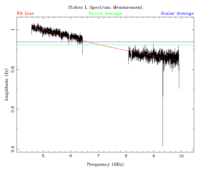
Source: 2244-372
Stokes I
Vector Average Amplitude:   9.237E-01         Phase:  -1.426E-06
             Uncertainty:   7.311E-01
Scalar Average Amplitude:   9.379E-01   Uncertainty:   7.211E-01
Vector Average Fit Coefficients:
 log S =   9.104E-02
       +  -4.980E-02 x (log f)^ 1
       +  -1.155E-01 x (log f)^ 2
Scatter around fit:   1.346E-02

And a plot that looks like:

The higher-order fit has a slightly smaller scatter around it (13.46 mJy) than does the lower-order fit (13.84 mJy). In the 16cm and 4cm bands, we make both order=1 and order=2 fits and choose the model that has the lowest scatter to go into the database. So, in this case, the best fit is:

$\log({\rm S} / 1 {\rm\,Jy}) = 0.09104 - 0.0498\log(\nu / 1 {\rm\,GHz}) - 0.1155\log(\nu / 1{\rm\,GHz})^2.$

The "Scatter around fit" value is entered into the database and gets used to estimate the uncertainty of any flux density derived from the model at a particular frequency. With regards to absolute flux density accuracy, simulations of randomly generated calibrators with various spectral indices shows that this measurement method reliably obtains better than 3% accuracy across the entire band regardless of which pair of frequencies is chosen, and so long as the calibrator has a signal-to-noise ratio of 50 or greater, which is not difficult to do over 4 GHz of bandwidth in a couple of minutes.

The "Vector Average Amplitude" and "Scalar Average Amplitude" are both entered into the database, and these values allow us to estimate the defect.

The uvfmeas task can also be used to determine the amplitude as a function of $uv$-distance, something that can be useful in determining if a source has structure, or if there is a confusing source in the field. However, if the source has a significant spectral index, then the flux density across the continuum band will change, and since different frequencies will lie at different $uv$-distances, this normal flux variation may be mistaken for structure or confusion.

A better idea is to plot the residual amplitude as a function of $uv$-distance. The residual amplitude is simply the flux density at a particular frequency minus the flux density model. For a non-confused point source with a good model, the residual amplitude should be zero (plus or minus the noise level) at all $uv$-distances. Using uvfmeas with the option uvhist makes the following plot:

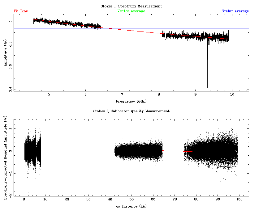
The bottom panel of the plot shows a point for each of the individual frequency channels at each time during the observation of the calibrator, after having the model flux density subtracted. Clearly, putting all those points into the database is not a viable option. Instead, uvfmeas determines the smallest and largest observed $uv$-distances, and makes 100 $uv$-distance bins to fit in this range. An average residual amplitude is calculated in each of these bins, and it is this histogram that is stored in the database. The red line on the bottom panel is the visual representation of this histogram, and for this calibrator you can see that it is very close to zero-valued at all $uv$-distances.

Measuring closure phase

The closure phase is measured for each calibrator using the Miriad task closure. Unlike for the flux density models, the closure phase is measured for each IF separately. For example, for an observation made in the 4cm band, we would run closure twice:


	      closure vis=1921-293.5500 stokes=i options=log device=/xs

	      closure vis=1921-293.9000 stokes=i options=log device=/xs

From the printed output of this task we take two values and keep them in the database, the measured and theoretical RMS for the closure phase, but this is unfortunately not an indicator of the closure phase itself. To get that, we need to actually read the log file that closure generates, that looks like:

Antennas 1-2-3
  32075.69531250      0.00747906
  32084.92773438      0.03184347
  32094.92773438      0.00064499
  32104.92773438      0.00748781
  32114.92773438      0.02183627
  32124.92773438      0.05054176
Antennas 1-2-4
  32075.69531250      0.01375755
  32084.92773438     -0.00359855
  32094.92773438     -0.00518243
  32104.92773438     -0.00782766
  32114.92773438     -0.00175100
  32124.92773438      0.01889207
	    ....

For each three-antenna set, the log has a time value in the first column (specified as the number of seconds after the start of the observation epoch) and the closure phase value in degrees in the second column. To obtain a single value for the closure phase we simply take each closure phase value on all baselines and take the average. This average closure phase is stored in the database.

Measuring miscellaneous parameters

There are several miscellaneous bits of information that the database stores that are useful to have, but can be a little tricky to obtain.

The source name, right ascension and declination of the observation, the time of the first and last cycles on source, the actual amount of integration time and the exact frequency configuration are all gathered from the uvindex task. This task is very easy to run:


	      uvindex vis=1921-293.5500

It produces output similar to the following:

Summary listing for data-set 1921-293.5500/

       Time        Source        Antennas Spectral Wideband  Freq  Record
                    Name        Calcode   Channels Channels Config   No.

12APR22:21:56:35.7 1921-293         n  6      2049        0      1       1
12APR22:21:57:24.9 Total number of records                             360

------------------------------------------------

Total observing time is  0.02 hours

The input data-set contains the following frequency configurations:

Frequency Configuration 1
  Channels  Freq(chan=1)  Increment  Restfreq     IFChain
    2049       4.47600    0.0010000   0.00000 GHz     1

------------------------------------------------

The input data-set contains the following polarizations:
There were 90 records of polarization YX
There were 90 records of polarization XY
There were 90 records of polarization YY
There were 90 records of polarization XX

------------------------------------------------

The input data-set contains the following pointings:
 Source       CalCode     RA            DEC             dra(arcsec) ddec(arcsec)
1921-293         n     19:24:51.06   -29:14:30.12           0.00         0.00

------------------------------------------------

The script that adds data to the database interprets the first and last times listed in the top section, and stores them in the database as MJDs. The total amount of integration time (accounting for flagging) is calculated by uvindex and is output as the "Total observing time" in hours.

The frequency configuration of the set is given as the number of channels, the frequency of the first channel and the frequency spacing between channels. From this we can tell which correlator mode was being used, and the sideband. Although this information is not readily available from the calibrator database web interface, it is stored and may be made available should it be required.

The source name, and the position it was observed at are shown in the bottom section of the uvindex output. The R.A. and Dec of each observation is stored separately to the nominal position of the calibrator, so we can tell if there is a discrepancy between the observed and "proper" coordinates.

To determine the array that was used for the observations we use the uvlist task:


	      uvlist vis=1921-293.5500 options=array,full

The output of this task looks like:

UV Listing for data-set 1921-293.5500/

Options: full,array

------------------------------------------------------------
Telescope: ATCA
Latitude:   -30:18:46.38
Longitude: +149:33:00.50
Mounts: Alt-az

Antenna positions in local equatorial coordinates

        X (meters)     Y (meters)     Z (meters)
        ----------     ----------     ----------
  1         0.0000         0.0000         0.0000
  2        -0.0209       -30.6222         0.0090
  3        -0.1162      -107.1460         0.0020
  4        -0.1710      -153.0710        -0.0010
  5        -0.3952      -352.0463         0.0140
  6        -5.1442     -4438.7747         0.0600

Antenna 1 is always listed at the origin in this output, but it is actually antenna 6 that never moves, so we begin by adding the required length to each position to make antenna 6 appear at (0, 0, 0). The X direction represents North-South (positive is North), and the Y direction represents East-West (positive is East). Since CA06 is always on station W392, and stations are numbered based on the station interval being 15.3m, it is straightforward to take these numbers and calculate which stations each antenna is on. In this case, CA01 is on W102, CA02 is on W104, CA03 is on W109, CA04 is on W112, CA05 is on W125 and CA06 is, as always, on W392.

A table of configurations is available, and with it we can match the array that was used. These stations correspond to the EW352 array.

Using the web interface

Front Page: Recent Database Changes

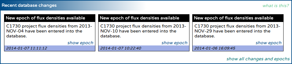
Each time the database is changed, a record is kept that summarises the change. Most of the time, this change will be a new epoch of measurements by the C007 or C1730 projects becoming available, but changes to calibrator position or recomputation of flux densities will also be tracked.

This section of the front page will always show the three most recent changes to the database. To get a full list of changes, and a list of all the measurement epochs in the database, click the "show all changes and epochs" link at the bottom right of the section.

For new measurement epochs, a "show epoch" link will be shown in the summary box; clicking this link will take you to a page that summarises the sources, bands and flux densities observed during that epoch.

Front Page: Quick-find Calibrator

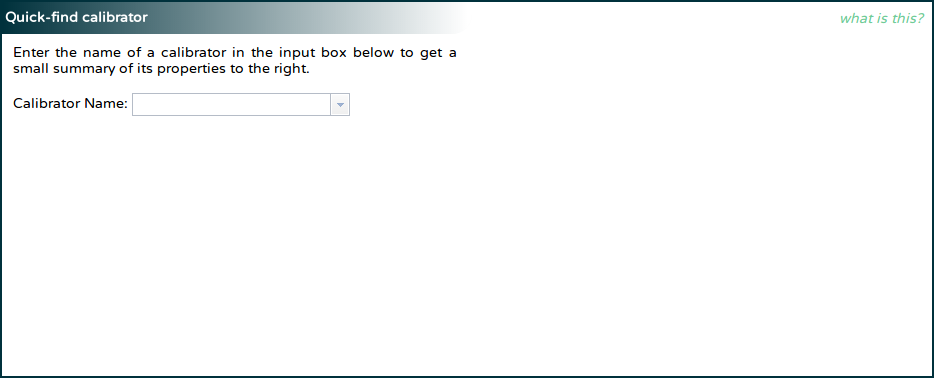
If you know the name of the calibrator you are interested in, and just want to get a quick summary of the latest flux density measurements in each band for that calibrator, you can very quickly get this information.

On the left of this section, you will see an input box asking for a calibrator name. As you enter the name of the calibrator, the input box will display the sources known to the database that match the entry you have made so far. You can select the source from the dropdown box or continue to type in the name yourself.

Once you have selected or typed the name of a calibrator in the left box, and pressed Enter or otherwise removed the focus from the input box, the interface will query the database. Once the results have come back from the server (which should occur in just a few seconds), the right side of the section should display the position of the calibrator, the rise and set LST at the ATCA, and the flux densities at some of the ATCA recommended continuum frequencies. If no observation of the source can be found in a particular band, the flux density for that band's recommended frequency will read "N/A" (not available).

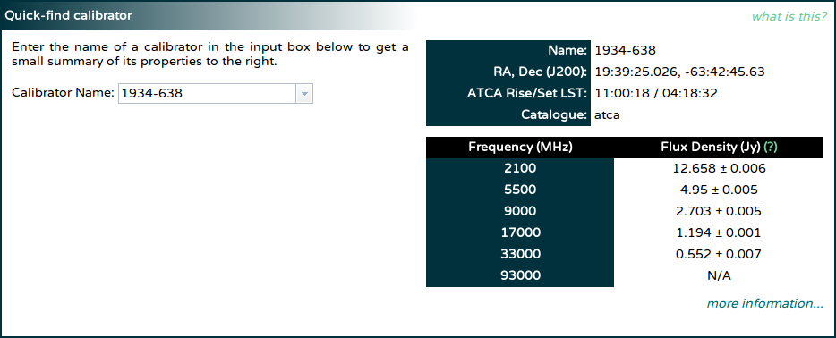
The "more information..." link at the bottom of the table of flux densities can be used to bring up a page that more contains much more information about the source.

Front Page: Search for Calibrators

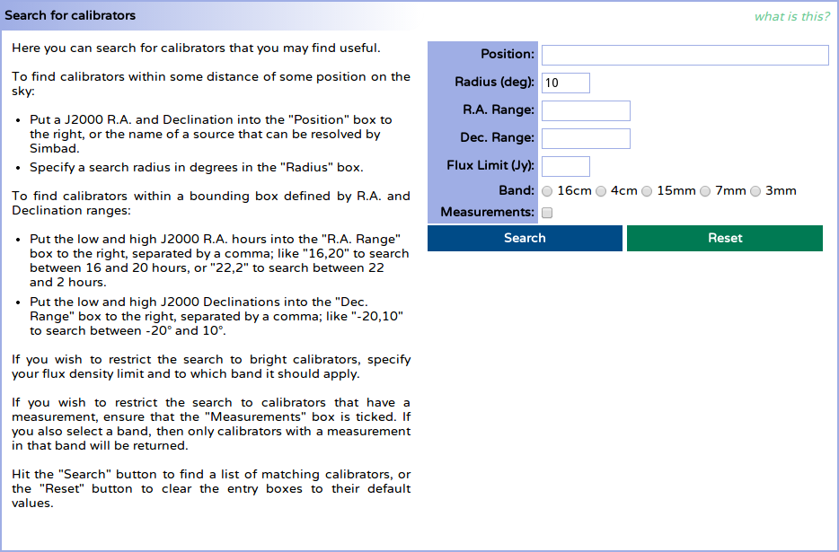
The instructions on the left of this section give a reasonable guide on how to search for a useful calibrator. This help section will thus be very brief, and will give only some more detail on the use of the "Position" box.

While entering a right ascension and declination (e.g. "19:39:25.026 -63:42:45.63") is a perfectly good way to use the "Position" box, most people are likely to be actually searching for calibrators around a known source rather than some arbitrary position. To make such a search easier, the "Position" box will detect if an entry looks unlike an R.A. / Dec. pair and then assume it is the name of an astronomical source which can be located with the help of the Sesame name resolver.

If you enter a source name then (e.g. "NGC 612"), and press Enter or otherwise take focus away from the "Position" box, you will get an animated box to let you know that the name is being resolved. Once the resolution has completed successfully, the box will be filled with the appropriate R.A. / Dec. (in this case "01:33:58 -36:29:36") and the animated box will turn solid green, and will show the name of the source that was just resolved. If the name resolution failed, the box will turn red, and will indicate the failure.

The "Search" button can now be used to search for calibrators around the position.

Change Page: Database Change Summary

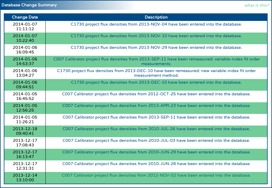
The change summary gives a full list of all the changes made to the database since its creation. Each change is given a small description, which is shown in this table. The time that each change was made is shown on the left of the table, and this time is in the local time zone (Sydney) will reflect daylight savings time if appropriate.

If the change relates to flux density measurements, then clicking on the description text will bring up a page that will show all the sources observed during the related epoch, and the flux densities measured in each band during that epoch.

If the change relates to a change in the details of a particular calibrator, then clicking on the description text will bring up a page that describes that calibrator, and the measurements in the database for that calibrator.

Change Page: Epochs

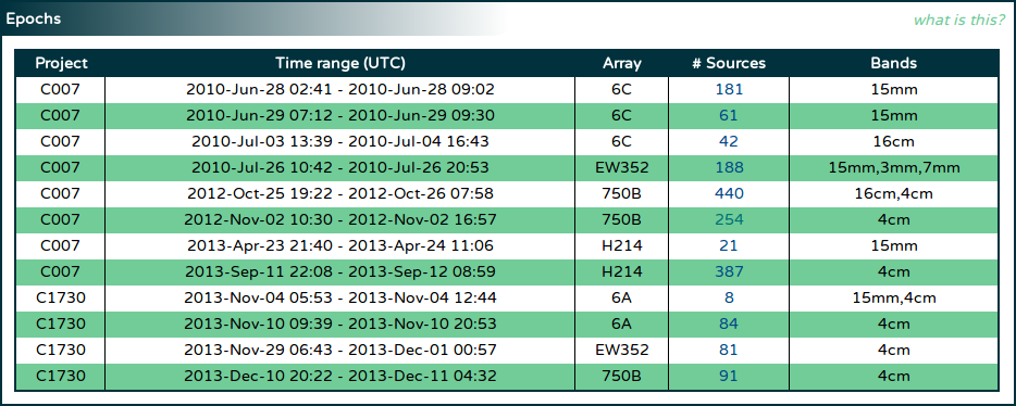
Since the majority of measurements in the ATCA calibrator database are obtained from the C007 and C1730 projects, this section is here to allow the user to easily see the epochs of these projects that have contributed data to the database.

The table itself will appear almost immediately after the page is loaded, and will be populated with a row for each of the epochs the database uses, with earlier epochs listed first. For each epoch, the project code it used, along with the full time range of observations and the array configuration at the time are given.

After the page has loaded, the table will begin to query the database for a more complete summary of each epoch (since this will take some time to compile). Sometime later, each row will also list the number of unique sources that were observed during that epoch, and the frequency bands that measurements were made in. Clicking the number in the "# Sources" column will bring up a page that will show all the sources observed during that epoch, and the flux densities measured in each band for those sources.

Epoch Page: Epoch Summary and Epoch Observations

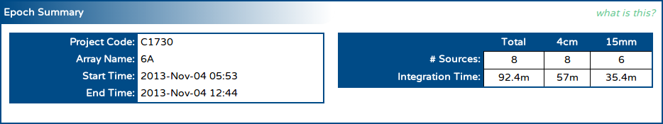
The epoch summary gives a very similar set of information to that found on the "Epochs" section on the change page: the project code, the array used during the observations and the epoch time range are all shown as soon as the page as loaded.

The page also queries the database for each source that was observed during the epoch, and then determines:

the bands that were observed in,
the number of unique sources that were observed in each band, and during the epoch as a whole (shown in the "# Sources" row in the table in the "Epoch Summary" section), and
the amount of integration time obtained over all the sources in each band (shown in the "Integration Time" row in the table in the "Epoch Summary" section).

After the sources that were observed in the epoch are found in the database, the table in the "Epoch Observations" section is shown.

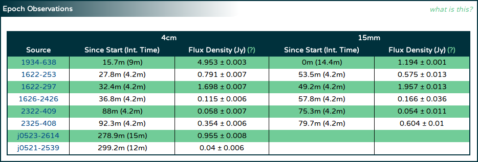
Lower frequency observations are shown to the left in this table. For each unique source that was observed, two columns are shown per band:

In the column labelled "Since Start (Int. Time)" are shown two values, the first being the time since the start of the epoch that the source was observed at in that band (in minutes), and the second (in parentheses) being the amount of integration time obtained for that source in that band (again, in minutes).
The flux density measured from this data, and its associated uncertainty in Jy, evaluated at the lowest recommended frequency in that band.

The sources are ordered in the table such that the sources observed first are listed first. Each source name is a link to a page that thoroughly describes the information that the calibrator database has about that source.

Search Page: Search Results

If you used the search section on the front page to find calibrators within some distance of some specified coordinate, the "Search Results" section might look something like the image below.

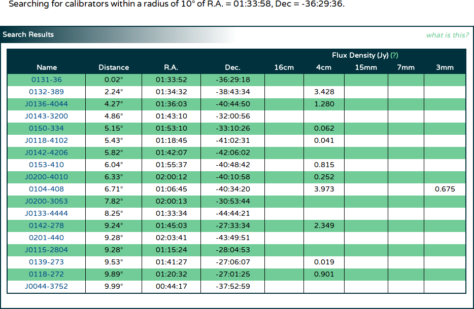
In the area above the "Search Results" section is a human-readable summary of how the interface interpreted the search parameters. After some time querying the database (during which time the message "Searching the database, please wait..." will be shown in place of the table shown in the image above), the table will appear with the search results.

The calibrators found that match the search query will be ordered by the distance to the specified coordinates, with closer calibrators listed first. The distance between the specified coordinates and each calibrator is given in the column labelled "Distance" in degrees. The R.A. and Dec. of each calibrator is given in the appropriately named columns, and each coordinate is rounded to the nearest arcsec for brevity. To look at more detailed information about a particular calibrator, click its name in the left-most column.

For each calibrator, the latest flux density in each band is found in the database, and listed in the appropriate column on the right of the table. If no flux density measurement has been made in a particular band, that column will remain empty.

If you searched for calibrators within a block of R.A. and Dec., the "Search Results" section might look like the image below.

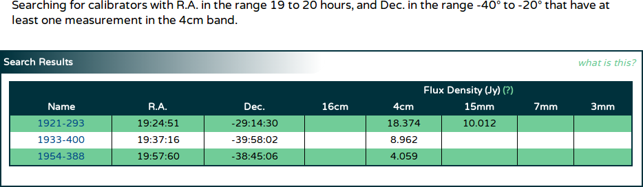
In this case, the "Distance" column is not shown, but in all other regards the tables are the same.

View Page: Source Information

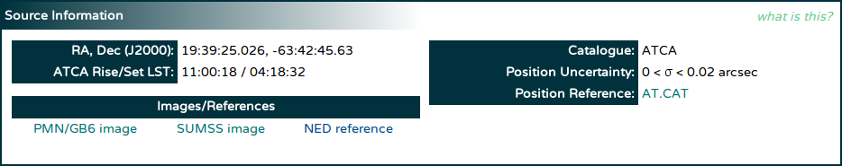
When viewing detailed information about a particular calibrator, the topmost section will be filled with basic information about the source, as shown above. The R.A. and Dec. of the source is shown, with the full accuracy available in the database, along with which catalogue it was taken from, the positional uncertainty, and in some cases, a link to the catalogue.

After the information is retrieved from the database, the web page itself calculates the LST when this source rises above the 12° elevation limit at ATCA, and the LST when it sets below the limit. These LSTs are shown in the "ATCA Rise/Set LST" row on the left.

For sources that have declinations -88° < δ ≤ -39°, -27° < δ ≤ -9° or 0° < δ ≤ 77°, a link will be made to NASA's SkyView service in order to quickly see an image of this source from the PMN/GB6 survey. This link will be in the "Images/References" table on the left;

For sources that have declinations south of -30°, a link will be made to SkyView in order to quickly see an image of this source from the SUMSS. For sources that have declinations north of -39°, a link will be made to SkyView in order to quickly see an image of this source from the NVSS.

A link will also always be made to the NASA/IPAC Extragalactic Database (NED) that will do a "near position" search around the calibrator's coordinates.

View Page: Notes

The database may have important notes about a calibrator, that may describe, for example, situations in which the calibrator might not be suitable. When the database has such notes, they will be shown in this section.

If the database does not have any notes for the calibrator being viewed, the text "There are no notes in the database for this source" will be shown in this section instead.

In some cases (usually when viewing a source from a C1730 epoch), you will be able to view the measurements made for a source that is not actually in the ATCA calibrator list. In this case, you will see the message "This source is not in the calibrator database". Any information shown about this source in the "Source Information" section will come from an actual observation at a specified epoch.

The warning for 16cm observers, seen at the bottom of the image above, will always be shown in this section.

If you are viewing information about a calibrator you know very well, and think that you have information about it that other observers should know, please feel free to send an email to the calibrators list with the information; we'd be happy to add it as a note into the calibrator database.

View Page: Flux Density Measurements

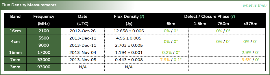
This table summarises the latest measurements made for this calibrator. For each of the ATCA frequency bands, the page will get the latest flux density model from the database, and evaluate it at one or more of the recommended frequencies in that band. The evaluated flux densities are shown in the appropriate row of the table, along with the UTC date that the model was measured at.

If no model can be found for a particular band for the calibrator being viewed, the flux density and date will be shown as "N/A" (not available).

The page will also get the latest defect and closure phase information for the calibrator being viewed in each band, and in each different array group. This information is shown in the "Defect / Closure Phase" columns on the right of the table. No date is given for each of these values, but one of the values shown will correspond to the same epoch in which the flux density model was measured.

View Page: Flux Density Request

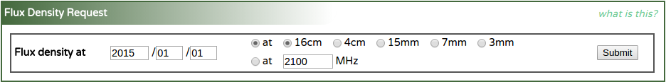
If you need to know the flux density of the calibrator you're viewing on a particular date in a particular band (or at a particular frequency), you can use this request facility to get this information.

To request the data, put the date of interest into the three input boxes on the left, with the year first, the month second, and the day of the month last. Then select the radio button for either the band you're interested in, or put a frequency (in MHz) into the frequency input box; make sure you've selected the correct "at" radio button as well. Once you've entered this information, press the "Submit" button on the right.

Shortly after you've hit the "Submit" button, you should get a table that looks like the image below.

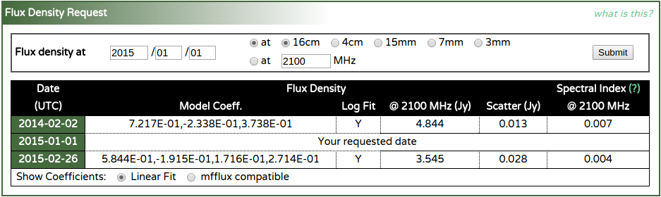
You will get information about the measurements closest in time to the date you supplied, with one before, and one afterwards. For each measurement, the coefficients of the flux density model that was measured are displayed, along with an indicator of whether the flux density model was made using the log of the flux densities and frequencies.

The flux density in Jy, evaluated at the frequency you supplied, or at the lowest recommended frequency in the band you requested, is also shown, along with the scatter around the fit as the uncertainty. Finally, the spectral index is shown, as evaluated at the same frequency as the flux density.

At the bottom of the panel, you may select whether you want the coefficients of a linear fit, or as the input that would be able to be used as the "flux" parameter in the mfcal task. You can read more about the way the flux density models are made here, in order to understand how to interpret these numbers. In the above example, the coefficients 7.217E-01,-2.338E-01,3.738E-01 should be interpreted as:

$\log({\rm S} / 1 {\rm\,Jy}) = 0.7217 - 0.2338\log(\nu / 1 {\rm\,GHz}) + 0.3738\log(\nu / 1 {\rm\,GHz})^2,$

where ${\rm S}$ is the flux density in Jy at the frequency $\nu$ in GHz.

The Miriad tasks mfcal, mfboot and gpcal don't understand the linear fit models like that shown above. Instead, they use a spectral index and curvature system, defined such that:

${\rm S} = {\rm S}_0 \times (\nu / \nu_0)^{\alpha(\nu)},$

where ${\rm S}$ is the flux density in Jy at the frequency $\nu$ in GHz, and ${\rm S}_0$ is the flux density in Jy at the frequency $\nu_0$ in GHz; we call this $\nu_0$ the reference frequency. The spectral index $\alpha(\nu)$ is defined to be:

$\alpha(\nu) = \alpha_0 + \gamma\times(\alpha_1 + \gamma\times\alpha_2),$

where

$\gamma = \ln(\nu / \nu_0).$

There is a fairly straightforward way of translating between the coefficients derived from a linear fit to the $\alpha$s needed by Miriad, and this is what occurs when you ask for the "mfflux compatible" coefficients.

From the mfcal help page for the "flux" parameter:

Key: flux
        Three to five numbers, giving the source flux density, a reference
        frequency (in GHz) and the source spectral index parameters.
        The flux and spectral index parameters are at the reference frequency.
        If no values are given, then MFCAL checks whether the source is one
        of a set of known sources, and uses the appropriate flux variation
        with frequency. Otherwise the default flux is determined so that
        the rms gain amplitude is 1, and the default spectral index is 0.
        The default reference frequency is the mean of the frequencies in
        the input data. Also see the `oldflux' option.

From the example above, the coefficients 7.217E-01,-2.338E-01,3.738E-01 translate into a "flux" parameter of 4.8437,2.1,0.0071,0.1623.

View Page: Measurement Details

To get a complete view of all the measurements that have been made of the source you're viewing, you can click on the "Show observation details" link at the top of the page, between the "ATCA Calibrator Database v3" title and the name of the source, as shown above. If you click this link, the page will reload, and after a short time you will get an additional panel - "Measurement Details" - which looks something like the image below.

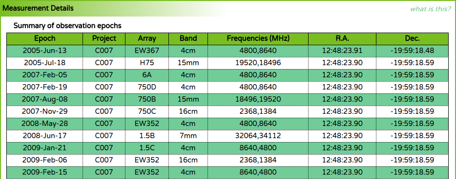
The top part of the measurement details panel shows a summary of all the observation epochs. A single line in the observation table will show the UTC date of the observation epoch, and the project code that observed this source on that date, along with the array configuration. Each line will only show a single frequency band, so if more than one band is observed for this source on a single date, you will see two lines with the same date. The central frequencies (in MHz) that were observed are shown, along with the R.A. and Dec. of the phase centre.

After the observation table, you will see the "Epoch Measurements" table, which looks something like the image below.

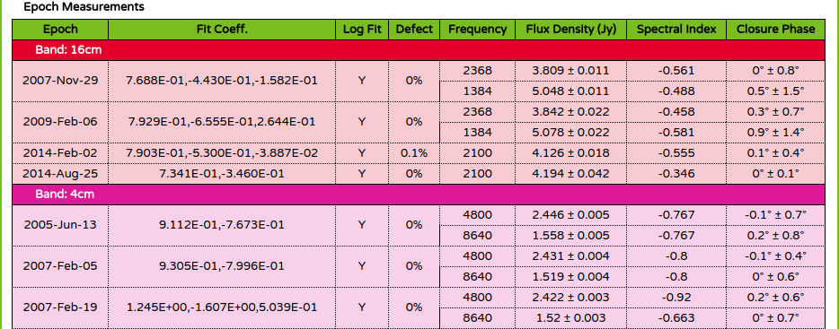
The measurements table is separated into frequency bands, so all the 16cm band observations are grouped together, as are 4cm observations, etc. In each band section, the individual measurements are listed in time order.

For each measurement, the observation epoch date is shown, and the linear fit coefficients (see here) are given, as is an indicator of whether the coefficients refer to a log-space fit. For each of the central frequencies that were observed for this measurement, the flux density (in Jy) and the spectral index at that frequency is shown. The closure phase measured in that band is also given.

Below this table is the "Measurement Statistics" table, as shown below.

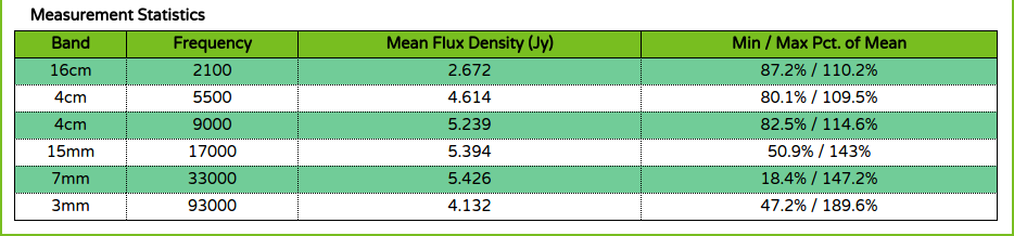
In this table, for each band and recommended frequency, the mean of all the measured flux densities is calculated and shown. The variation of all the measurements away from this mean is then calculated and shown as a minimum and maximum percentage of the mean value. This can be used as a good estimate of the variation of this source over time.

View Page: Flux Density Time Series

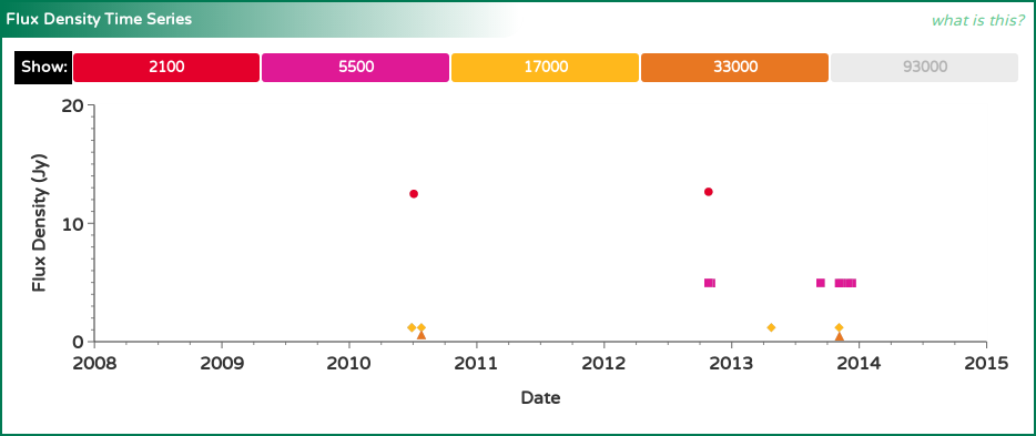
This plot shows how the flux density of the calibrator has changed over time in each of the ATCA frequency bands. Because the flux densities in the calibrator database are actually represented as models fit to the data during the measurement procedure, the flux densities can be evaluated at a consistent frequency regardless of the frequencies actually observed in any epoch (in the same band). This allows us to do a much more accurate comparison between flux densities measured in multiple epochs.

In the plot above we see that the flux density of this calibrator (1934-638 in this case) is different in each of the bands (as expected). Since the flux density of the calibrator would be different depending on the frequency, only a single frequency is chosen per band, and these frequencies are shown at the top of the plot next to the "Show" label, in MHz.

Since there are many plots on the calibrator view page, a consistent colour scheme is used across them all.

Band Name	Colour	Symbol
16cm	Vermillion	circle
4cm	Fuchsia	square
15mm	Gold	diamond
7mm	Orange	triangle
3mm	Plum	inverted triangle

Each of the buttons in the legend next to the "Show" label is coloured if there is data on the plot in that band. If there is no data available to plot in a particular band, that band's button will be coloured grey. Clicking a band's button (if it is not coloured grey) will remove the data from that band from each of the plots on the view page, and the button will then appear slightly transparent (but will still have the same band colour). To add the data from that band back to the plots, click the band button again.

When the data shown on this plot changes (as bands are added or removed from it), the y-axis range will change to keep all the data comfortably on the plot. The x-axis range is fixed, regardless of the epochs that are actually available for this calibrator.

View Page: Spectral Index Time Series

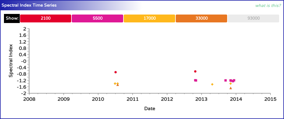
This plot shows how the spectral index of the calibrator has changed over time in each of the ATCA frequency bands. Because the spectral indices are computed from the flux density models in the calibrator database at a consistent frequency, the spectral index should stay reasonably constant with time, unless physical changes in the calibrator cause the emission mechanism to vary, or the flux model is inaccurate.

In the plot above we see that the spectral index of this calibrator (1934-638 in this case) is different in each of the bands (as expected since 1934-638 is a GPS source). Since the spectral index of the calibrator would be different depending on the frequency, only a single frequency is chosen per band, and these frequencies are shown at the top of the plot next to the "Show" label, in MHz.

Since there are many plots on the calibrator view page, a consistent colour scheme is used across them all.

Band Name	Colour	Symbol
16cm	Vermillion	circle
4cm	Fuchsia	square
15mm	Gold	diamond
7mm	Orange	triangle
3mm	Plum	inverted triangle

When the data shown on this plot changes (as bands are added or removed from it), niether the x-axis or y-axis range will change, as they are both fixed.

View Page: Flux Model

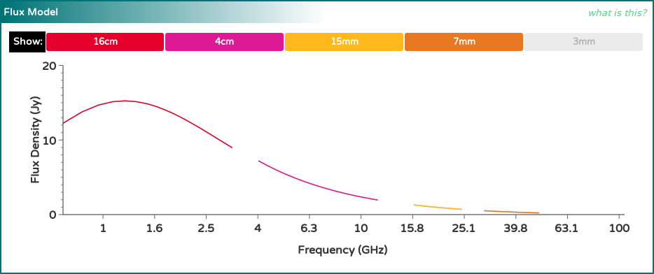
This plot attempts to illustrate the latest flux density models that have been measured for this calibrator. It does this by evaluating the flux density models measured in each band (in the most recent epoch they were obtained) at several frequencies across the band, and a line is drawn between these points.

In the plot above we see that the flux density models of this calibrator (1934-638 in this case) are different in each of the bands (as expected), but they seem to join quite smoothly together. This is what is expected for a calibrator that has a constant flux density with time. If however the calibrator is varying, the flux models may appear quite disjoint from one another, unless the models in each band were made from epochs closely spaced in time.

Since there are many plots on the calibrator view page, a consistent colour scheme is used across them all. The following table shows the colours that represent each band, and also the frequency range that the models are evaluated over.

Band Name	Colour	Symbol	Freq. Range (MHz)
16cm	Vermillion	circle	700 - 3300
4cm	Fuchsia	square	4000 - 12000
15mm	Gold	diamond	16000 - 25000
7mm	Orange	triangle	30000 - 50000
3mm	Plum	inverted triangle	85000 - 105000

When the data shown on this plot changes (as bands are added or removed from it), the y-axis range will change to keep all the data comfortably on the plot. The x-axis range is fixed to contain the entire range of frequencies shown in the table above, regardless of frequency bands that are actually available for this calibrator. The x-axis is also shown logarithmically.

View Page: Structure Plot

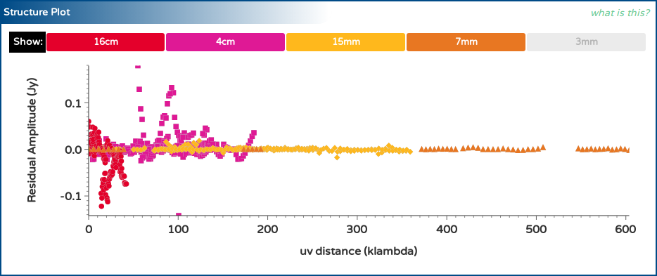
This plot shows the histogram points measured by the uvfmeas task in each epoch, as described in the section regarding the measurement of flux models above. For each band, the five most recent histograms are obtained from the database and shown here.

For a good calibrator, we expect that the residual amplitude should be zero at all $uv$-distances. The plot above does not show this to be the case for 1934-638, which we know is a good calibrator. Looking at the colours of the points that deviate from zero shows that short baselines at low frequencies are the biggest outliers. This can be attributed to low-level RFI in the most part, as the deviations do not exceed 0.2 Jy for a source that is much stronger than 3 Jy over most of the frequency range that we see deviations for.

Our general recommendation for interpreting this plot is to look for significant deviations (usually much larger than 1% of the source flux density) and to be concerned only if the deviations seem to have a recognisable pattern to them. In the plot above, the deviations are semi-random with plenty of discontinuities.

Interpreting the measurements

Flux Densities

Flux densities are shown by the calibrator database either at a particular frequency (such as on the calibrator-specific page) or in a particular band (such as on the epoch view pages). The flux densities are obtained by evaluating the model that was fit to the visibilities during the data reduction at a specific frequency. On some pages this frequency is explicitly specified, but when only the band is specified, the frequencies are set to be the lowest recommended frequency in that band, as shown in the following table.

Band Name	Evaluation Frequency (MHz)
16cm	2100
4cm	5500
15mm	17000
7mm	33000
3mm	93000

For example, the model measured for 1934-638 during the 2010-JUL-03 epoch (in the 16cm band) is:

$\log {\rm S}(\nu) = 1.180 + 0.1769\times\log \nu - 1.355\times(\log \nu)^2,$

where $\rm{S}$ is the flux density in Jy, and $\nu$ is the frequency in GHz. Thus, if the 16cm flux density is specified on one of the calibrator database pages, it is derived from:

\[\begin{eqnarray} {\rm S}(2.1) & = & 10^{1.180 + 0.1769\times\log(2.1) - 1.355\times(\log(2.1))^2} \\ & = & 12.483 {\,\rm Jy} \end{eqnarray} \]

Each flux density is usually accompanied by an uncertainty after a $\pm$ symbol. For example, the flux density above would usually be given as $12.483\pm0.002$ Jy. This uncertainty comes from the RMS value of the visibility amplitudes after the measured fit is subtracted.

On all pages where the flux density is shown as a number, both it and the associated uncertainty are rounded to the nearest mJy.

In general, observations made by the C007 calibrator project will reach sensitivities of around a few mJy. If the scatter around the fit is observed to be more than 10 mJy, the associated flux density should be treated with some suspicion. If the scatter is more than 100 mJy then the flux density is probably incorrect, as there will likely have been some problem with the data.

Defects and Closure Phases

The defects and closure phases displayed in the "Flux Density Measurements" section on the calibrator page give an indication of the suitability of the source for calibration purposes.

During the flux density measurement process, both the scalar-averaged and vector-averaged flux density is measured for each band as a whole. We assume that the vector-averaged flux density represents primarily the flux present within the resolution element at the phase centre of the observation, which is set to be the known position of the calibrator. The scalar-averaged flux density should represent the amplitude response of the primary beam, which is not restricted to the source at the phase centre, and should always be equal to or larger than the vector-averaged flux density.

The defect is defined to be:

${\rm defect} = ( [{\rm S}_{sca} / {\rm S}_{vec}] - 1)\times 100\%,$

where ${\rm S}_{sca}$ is the scalar-averaged flux density, and ${\rm S}_{vec}$ is the vector-averaged flux density.

But the defect itself is not a good summary of a calibrator's quality, as there could be a number of reasons for a non-zero defect (which we'll describe later). For this reason, we measure another quantity during the reduction process: the closure phase. If there is a point-like component in the field then the average closure phase measured by each set of three antenna should be zero for that component, regardless of the position of the component within the field. If the component is not point-like, then the closure phase will be non-zero.

Of course there may be more than one component in the field, but brighter components will influence the measured closure phase more than fainter components.

Taken together, the defect and closure phase gives us an idea of what the calibrator field may be like, as summarised in the following table.

Defect	Closure Phase	Interpretation
small	small	A dominant point source at the phase centre; little to no confusion.
moderate	small	Probable confusing source within the field, bright enough to cause issues with calibration.
large	small	Either a confusing source with a very similar brightness to the source at the phase centre, or likely to be a point source offset from the phase centre (i.e. a calibrator observed at the wrong position).
moderate - high	moderate - high	Significantly resolved structure bright enough to make calibration very difficult.

To assist with the use of these classifications, the defects and closure phases are colour-coded where they are displayed. "Small" defects and closure phases are coloured green, "moderate" values are coloured orange, and "high" values are coloured red.

Since a "point-like component" is simply a source of flux density that is unresolved by the interferometer, it is clear that the definition is dependent on the interferometer's resolving power. This is why the defects and closure phases are reported for various array sizes. These values come only from arrays with maximum baselines less than or equal to the length given in the header above the column. For example, values given in the column headed by "1.5km" come only from 1.5 arrays (1.5A, B, C or D). You should use the numbers corresponding to the array you plan on using in assessing the suitability of a particular calibrator.

Spectral Indices

Spectral indices are shown by the calibrator database at a particular frequency, which is usually listed near to the spectral index value itself. The spectral indices are obtained by evaluating the derivative of the model that was fit to the visibilities during the data reduction at this particular frequency.

We define the spectral index of a source by noting that for most sources the observed flux density is dependent on the observing frequency via

${\rm S} \propto \nu^{\alpha},$

where ${\rm S}$ is the flux density at some frequency $\nu$, and $\alpha$ is the spectral index. We define $\alpha$ such that negative values indicate that the flux density decreases with increasing frequency.

Measuring a source's spectral index is thus generally achieved by measuring $\log {\rm S}$ at multiple $\log \nu$ and fitting a line, of which $\alpha$ is the slope. But this is not always possible. The calibrator database stores models with up to 3 coefficients in each of the models:

\[\begin{eqnarray} \log {\rm S} & = & a + b\times \log \nu + c\times(\log \nu)^2 \\ {\rm S} & = & a + b\times\nu + c\times\nu^2 \end{eqnarray} \]

The logarithmic models are used for the vast majority of the calibrators in the database, but for those calibrators with flux densities near zero (and thus with flux densities in a particular channel that may be negative), the non-logarithmic models are used.

The spectral index is just the rate of change of $\log {\rm S}$ with $\log \nu$, which is easy to compute for the logarithmic model:

$\alpha \equiv d\log{\rm S}/d\log\nu = b + 2c\times\log\nu.$

It is straightforward to see that if $c = 0$, then $\alpha = b$ as expected.

For the non-logarithmic model, we first have to do some substitution:

$\log {\rm S} = \log (a + b\times\nu + c\times\nu^2).$

If we call $x \equiv \log\nu$, then $\nu = 10^x$, and the equation above becomes:

$\log {\rm S} = \log (a + b\times10^x + c\times10^{2x}).$

We can take the derivative of this now (thanks to Wolfram Alpha):

$\alpha \equiv d\log {\rm S}/dx = 10^x(b + 2^{x+1}\times5^xc)/(a+10^x(b+c10^x)).$

This can be further simplified by reversing the previous substitution and identifying the denominator as simply the equation for the flux density:

$\alpha = \nu(b + 2\nu c) / {\rm S}$

We note that the non-logarithmic models may be non-physical, as they allow for negative flux density, but should suffice for how they are used here, as the noise level on observations where they are used is large enough to make it the dominant form of the uncertainty.

VLA Calibrator Information

For those calibrators that are also in the VLA calibrator list, the calibrator database page will show the appropriate entry from the VLA calibrator manual.

The information contained in the calibrator list is very compact, but conveys a significant amount of information. A key to the intepreting the information is given on this page.