Information for Mopra Observers

Introduction
The Mopra 22-m antenna is part of the Australia Telescope National Facility (ATNF), operated by the CSIRO. It is used together with other AT antennas (the six 22-m dishes at Narrabri, and the 64-m Parkes dish) as part of the Australian Long Baseline Array. It is also used on its own, for single-dish observations, particularly at millimetre wavelengths.
The telescope is at latitude -31° 16' 04''.451, longitude +149° 05' 58''.732 (east of Greenwich), and its height above sea level is 850 m.
As part of a major upgrade program, millimetre receivers covering 3 bands between 16 and 116 GHz and the MOPS backend system were installed at Mopra between 2004--2008. The backend produces two 8-GHz bandwidth IFs from each polarisation, and is capable of observing several spectral lines simultaneously. Observing at 3-mm is best in the APR term only (winter months).
Information on applying for telescope time is available online in the ATNF Guide. Be sure to first check the current status.
From October 2012, Mopra is being operated under a new model, with the provision of funding from the National Astronomical Observatory of Japan, the University of NSW, and the University of Adelaide allowing for the the continued operation of the telescope, with these groups being provided with guaranteed observing time in return.
A severe bushfire on Sunday January 13, 2013 burned a large region near Coonbarabran including the Mopra and Siding Spring Observatories. Fortunately, the telescope itself and the key data-taking equipment were spared by the fire, but mains power was cut and the on-site building suffered significant damage. The telescope was returned to operations in May 2013.
Mopra control desks are situated in Science Operations Centre at Marsfield (Sydney), and the control building of the Australia Telescope Compact Array located at the Paul Wild Observatory near Narrabri. Observers must carry out their own observations. Full remote observing from anywhere in the world is available for suitably qualified observers.
If you have a query about the Mopra telescope then send an email to mopra-sciops @ atnf.csiro.au .
Receivers
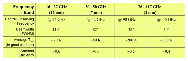
Mopra is equipped with three receivers for single-dish observations. These are:3-mm band covering 76 to 117 GHz
7-mm band covering 30 to 50 GHz
12-mm band covering 16 to 27 GHz
The receivers use Indium Phosphide (InP) High Electron Mobility Transistor (HEMT) Monolithic Microwave Integrated Circuits (MMICs) as the amplifying elements. The receiver systems require no tuning and include noise diodes for system temperature determination. (Note that the 3-mm system also requires an paddle/vane measurement for the system temperature determination).
The following table summarises the parameters for the three receiver systems.
MOPS - Mopra Spectrometer
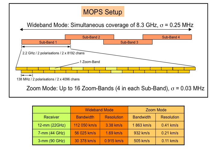
MOPS was funded in part through a grant instigated by the University of New South Wales (UNSW) under the Australian Research Council Grants scheme for Linkage, Infrastructure, Equipment and Facilities (LIEF), and in part by CSIRO-ATNF. Commissioning was carried in Oct 2005.MOPS is a digital filterband. The 8-GHz broadband signal channels from the mm receivers are transmitted to MOPS, installed in the Mopra equipment room, via broad band analogue fibre optic links. Each 8-GHz IF is then split into four 2.2-GHz bandwidth channels and down converted to the base band. Every 2.2-GHz base band IF signal is digitised by a 2-bit 4.4 Gsample/sec Indium Phosphide digitiser. The digitisers were developed at ATNF and fabricated at TRW in March 2000, under the CSIRO Special Executive program.
MOPS offers two configurations:
Wideband Mode
In Wideband Mode continuous coverage over 8.3 GHz is achieved
using 4 overlapping sub-bands. Each sub-band is 2.2 GHz wide with 2 x
8096 channels (1 x 8096 chans for each polarisation, xx and yy). Each
dataset contains a total of 64 768 channels (4 x 8096 x 2). The label
for this mode is mops_2208_8192_4f. You may choose a binning mode
identified as mops_2208_1024_4f (not popular but will help save disk
space since it reduces the sizes of your data files).
Zoom Mode
In Zoom Mode it is possible to observe up to 16 zoom bands (often
referred to as "windows") simultaneously. Each zoom band is 137.5 MHz
wide and has 2 x 4096 channels (1 x 4096 chans for each polarisation,
xx and yy. Up to four zoom bands may be selected in each of the 4
overlapping sub-bands. The label for this mode is mops_il_zoom.
The following diagram depicts a typical arrangement of bands within
the 8 GHz frequency range.
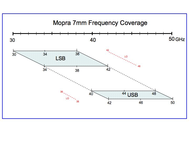
Additional information for 7-mm observations
The figure illustrates the frequency coverage of the 7-mm observing band on Mopra. Every frequency from 30 to 50 GHz is observable, but with some limitations. There are hardware limitations in the LO chain that have resulted in limitations in the tuning ranges for MOPS. The tuning ranges (specified as the band centre) are:34 to 38 GHz
44 to 46 GHz
At any frequency within these ranges the full 8-GHz frequency coverage is possible. The gap between 38 to 44 GHz cannot be processed as one frequency setting.
For example, when tuned to 38 GHz your frequency band will cover the range 34 to 42 GHz. When tuned to 44 GHz the frequency band will cover the range 40 to 48 GHz. However, one cannot have a band containing 38 to 44 GHz.
Additional Technical Information
Mopra Parameters
A new sensitivity calculator has been developed for the 12-, 7- and 3-mm bands. The calculator is only suitable for position-switching mode. The on-the-fly mapping mode will be implemented at a later data. In the mean time you will have to use the 2005 on-the-fly calculator.Observing Modes
Two observing modes are possible with Mopra:1. Position Switching Mode
This mode moves the telescope back and forth between the target position (ON) and a position offset from the target (OFF), recording a spectrum at each position. The spectrum at the OFF position is labelled as a "reference spectrum" and is used in a quotient calculation (performed offline) to produce a target spectrum that has no telescope/sky contribution. It is very important that the OFF position does not contain any line emission. The primary advantage of this mode is that it produces spectra with flat baselines. The primary disadvantage is the amount of time lost slewing the antenna back and forth between the ON and OFF positions. Two different OFF-ON patterns are possible: The symmetric pattern OFF-ON-ON-OFF has the advantage of reducing antenna drive times. The asymmetric pattern OFF-ON-OFF-ON ensures that both the ON and the OFF spectra are observed through the same patch of sky.
An on-line tool is available on the Mopra web page for the creation of position-switching schedule file. To reduce position-switching data use ASAP.
2. On-the-fly Mapping (OTF)
On-the-fly (OTF) mapping is the optimal method for spectral line imaging. In this mode, also called raster mapping, data is continuously taken while scanning along a row between predefined points A and B. A map is constructed by stacking several different rows. Each row is separated by less than the FWHM beamwidth. At the end of each row a single pointed observation at an OFF (reference) position is required. The OFF position is several arcmin from the mapped area. The OFF spectrum is used for offline/sky continuum subtraction. This is a very efficient mode of observing as it reduces the number of OFF positions to a minimum and uses drive times for data acquisition. The scanning speed is limited by the number of seconds to average spectra over before writing to disk. For Mopra this value is currently fixed at 2 s. On-the-fly mapping is recommended for mapping regions larger than about 2 arcmin x 2 arcmin as it reduces overheads, is easy to observe and the data reduction is straightforward.
An on-line tool is available on the Mopra web page for the creation of an On-the-fly map schedule file. To reduce on-the-fly mapping data use Gridzilla/Livedata.
For additional information take a look at the presentation from the Mopra Training Day held in March 2008 - Observing Modes.
Calibration
Flux Temperature Scale
For MOPS spectra there are two flux temperature scales:
1. Corrected antenna temperature (Ta*)
This is the power detected
by a telescope expressed in terms of an equivalent blackbody
temperature. Ta* should be corrected for systematic effects of the
Mopra system (receiver noise, back scattered radiation, side lobe
contributions, ohmic losses etc, all of which are incorporated into a
Tsys measurement ) as well as the affects as atmospheric attenuation,
Tau. This temperature scale is essentially the Mopra temperature
scale and is what comes out of the MOPS box.
2. Main Beam Brightness Temperature (Tmb)
This is the calibrated
antenna temperature after correction for the main-beam efficiency of
the telescope. Tmb will be the true source brightness temperature of a
source that just fills the main beam. This temperature scale is
essentially a telescope-independent temperature scale. It allows one
to compare data taken with Mopra with data taken with, for example,
APEX.
To convert Ta* to Tmb you need to divide by the antenna efficiency. For characterisation of the 12-mm and 7-mm efficiency, see the paper by Urquhart et al. 2010. For details on the antenna efficiency in the 3-mm band refer to the article by Ladd et al. 2005.
System Temperature
The Mopra receivers are equipped with a noise diode to measure the system temperature. The values of the system temperature are updated online and these values are fed into determining the flux scale of the output spectra from MOPS (Ta*). The system temperature measurement does not take into account the attenuation of the spectral emission line caused by the atmosphere. Currently for Mopra we only make corrections for this atmospheric attenuation (tau) in the 3-mm waveband. This is done using the paddle/ vane method (Ulich & Haas 1976). This method is "hard-wired" in the MOPS online data-flow system, which means that all 3-mm Mopra data must include a paddle measurement. The advantage of the paddle method is that it is fast and better-suited to changeable weather conditions. In good weather conditions the system-temperature measurements (updated continuously via a noise diode) are updated with a new tau correction (using a paddle measurement) every 20 mins.An alternate method for measuring tau is to use a skydip procedure whereby the gated total power (GTP) is measured at several different elevation settings. The change in GTP with elevation yields a measurement for tau. The skydip method is time consuming (~ 10 mins to complete) and is only suitable for very stable weather patterns (cloud-free skies). Skydip measurements are not straightforward with the Mopra system and are currently not supported.
Currently for Mopra there is no atmospheric correction made in the 7- and 12-mm bands, either online (with paddle or skydips) or offline (using an atmospheric model). For 12-mm and 7-mm Mopra observations the effect of the tau correction to the line signal strength is expected to be less than 25% and combined with the other flux uncertainties (pointing, antenna efficiency etc) this is not significant.
Note: For ATCA the tau correction at 12- and 7-mm is made offline during the data reduction process. There is a Miriad routine that uses a simple atmospheric model to determine tau and then scale accordingly the 7-mm and 12-mm visibilities. No online paddle measurement is made. There is a command in Miriad that lets you play with the atmospheric model to gauge what the tau correction is for certain temperature/pressure/humidity readings. The task is called "opplt". For Mopra, the plan is to eventually incorporate the miriad opacity model into ASAP so that corrections can be done for the 7- and 12-mm bands.
For additional information take a look at the presentation from the Mopra Training Day held in March 2008 -Temperature Scale and Flux Calibration.
Mitigating the baseline ripple
For observations with an on-source integration time greater than about 10 minutes the spectra are dominated by a 30 MHz baseline ripple. This baseline ripple can dominate the rms noise and is a real problem for science projects that are looking for detections of weak lines. The baseline ripple is the result of a standing wave between the Mopra dish and the subreflector. There are a couple of online observing and offline data reduction techniques that observers can try out in order to minimise the ripple.
Of course in bad weather (e.g thick clouds) even spectra with short
integration times will suffer from baseline ripples because of the
change in sky continuum levels as the clouds pass overhead. In this
situation keep the time difference between the on-source and
off-source observations as short as possible (e.g. 30 sec) or consider
stopping all observations until the weather improves.
Online Approach - Median Reference Spectrum
One technique that seems to have some success involves a non-standard
way of doing position-switching whereby two spectra at different
reference positions (also called "sky" or "off" positions) are taken
and then averaged together to form a median reference spectrum. This
median reference spectrum is then used in the quotient calculation. The
reasoning behind this method is that the ripple is exasperated by the
difference in continuum levels between the target position and the
off-source (reference) position. By using two different reference positions and
then combining them together to form a median reference spectrum there is a
better chance of matching the continuum levels with that of the
target. Unfortunately this method involves quite a bit of fiddling
with the schedule files and the data reduction.
Currently the schedule preparation tool on the web only permits the following sequence: REFERENCE/TARGET/REFERENCE/TARGET or REFERENCE/TARGET/TARGET/REFERENCE. So the way to proceed is to decide on your two reference positions (e.g. offset on either side of your target), then make your schedule files with the web preparation tool but only enter one of the reference positions. Save the output (a text file) and then edit directly the text file to include your second reference position (e.g. REFERENCE#1/TARGET/REFERENCE#2/TARGET)
Data reduction for position-switching mode is done with the software package ASAP. To perform a non-standard quotient calculation on the data requires some python knowledge . A tutorial is available online that may help you (Tutorial 6). The tutorial uses Parkes multibeam data to extract a median reference spectrum.
Note that you will still be able to reduce your data with ASAP in the
standard way (with no median reference spectrum). It is always worth
using this standard method first for a quick look at the data and to
experiment with the lagflag procedure (see next paragraph). You may
find that the lagflag procedure is sufficient for your data. In which
case you do not need to create a median reference spectrum and
calculate the quotient manually. Unfortunately you won't know this
until you have already taken and looked at your data, which is why it
is a good idea to take data using two different reference positions,
just in case.
Offline Approach - Flagging the Lag Spectrum
Another way to reduce the affect of the baseline ripple is to fourier
transform the spectrum and flag the data in frequency space. It is
possible to do this in ASAP using the "lag_flag" command. A tutorial
is available online that may help you
(Tutorial 5). The best result is found using the following input parameters:
c.lag_flag(12,11.9999,unit="MHz")
Schedule Files
The schedule is intended to mimic the operations on the GUI - you enter some new fresh parameters (eg, a new source position), and launch operations (e.g.,a scan). Any GUI command can be included in the schedule. Once a schedule has been invoked ("start") the schedule maintains control of TCS, shutting outmost of the user-selectable functions of the GUI.
A schedule contains a loose mix of parameters and actions; these are grouped in UNITS. The recommended procedure is to make each unit self-sufficient; each unit may contain a number of actions, and each action will be governed by all the parameters between the start of the unit and the action. TCS reports the number of actions and units in a schedule; the schedule pointer increments on data collecting actions, not units. It is therefore in practice simpler to write schedules containing precisely one action per unit (though unit-based incrementing may be introduced in the future).
When the user requests TCS to start an observation by clicking on the "start TRACK"/"start SCAN" button on the main action panel (without using a schedule), TCS reads all the parameters from the GUI and uses these to define the observation. When a schedule is used, by clicking on the "Start sched" button, TCS first reads all the GUI parameters, then steps through the schedule from the nominated starting point. Any parameter defined in the schedule will therefore override the GUI value. Further, the value displayed on the GUI will be immediately reset to the value defined in the schedule, so the new value persists indefinitely (until explicitly changed). Thus the GUI should represent accurately the parameters of any observation currently in progress. (If this fails to occur it is a reportable bug!). A further important consequence of this model is that parameters not specified by the schedule will default to the value displayed on the GUI. This is important to bear in mind, particularly at the start of an observing session. Unintended settings on the GUI inherited from a previous observing session can be disastrous if not detected by careful checking!
An observer can use TCS without ever using a schedule. For example, a series of repeated or similar simple observations of a list of sources might be accomplished more easily from the GUI alone, loading the source details from a user-prepared catalogue. This is the most interactive but also the most flexible style of observing.
The next level is to write a "minimalist" schedule containing only those commands which change from one observation to the next (e.g. source details) and use the GUI for fixed parameters or those which change only occasionally (e.g. correlator configuration etc).
Alternatively, an observer can "play it safe" and include in the schedule file every relevant setting in every "unit". This gives protection against inheriting unwanted settings. It also has the advantage that the schedule files can be started midway through (simply specify the start "unit" number in the TCS).
A hybrid scheme is to define all or most of the relevant parameters in the first "unit" of the schedule, and thereafter specify only changes to parameter settings (rather than repeating them for every integration). This can be a very convenient mode of observing, but beware of re-starting a schedule midway through after an interruption - any GUI parameters that have been changed in the meantime may not get reset if you skip the first integration of the schedule.
The easiest way to create a schedule file is to use the on-line scheduler tools. There are two different schedulers - one for Position Switching and one for On-the-fly mapping. Links to the latest versions of the schedulers are on the main Mopra webpage. Both schedulers use the hybrid scheme (defined above). These schedulers create a text file that should be first saved to your local machine (filename.sch).
It is possible for users to create their own schedule file (without using the on-line scheduler tools). Refer to the TCS User Manual for more information on individual commands.
Once your schedule file is complete it must be uploaded to a local machine called bigrock, which runs the Mopra Telescope Control Software (TCS). On bigrock there is the directory /nfs/online/local/tcs/sched/2013. In this directory you must first create a directory using your Mopra project number (e.g. M007) and then upload all your schedule files to this new directory. Please note that there is no read/write protection or guaranteed backup of observer schedule files on bigrock.
Catalogue Files
If you have a large target sample you may prefer to use a catalogue file, which lists all the source names and coordinates. The catalogue file can then be used in conjunction with a generic schedule file, which does not include entries for the source name and coordinates. Here is an example of the format of a catalogue file. Here is an example of generic schedule file that does a simple position-switch observation with a 3-mm paddle calibration.
Note that it is not possible to use a catalogue file in conjunction with a schedule file that specifies the reference position using absolute co-ordinates. Only offsets are permitted.
Currently there is no generic schedule file that does on-the-fly mapping. For this observing mode a centre position must be specified in the schedule file. (A catalogue file cannot be used.)
Data Reduction
For position-switching data use ASAP. A tutorial for ASAP beginners is now available (May 2008). More tutorials will be added.
An ASAP-GUI interface has been developed by Cormac Purcell and is available for download. This GUI is useful for quick-look data reduction of position-switching data. It also has the capability to export the reduced data. To start the GUI type "python -i QuickData.py". Load in your data files with the "Browse" and "Load" buttons. Select the IF you wish to work on with "Current IF". First average in time the data for each of the two polarisations (2 blue boxes) and then average the two polarisations (2 green boxes).
For on-the-fly mapping use Livedata/Gridzilla. New users should use this worksheet.
Telescope Control & Monitoring
For the time being take a look at the presentation from the Mopra Training Day held in March 2008.Telescope Control & Monitoring.
Computing & Data Handling
For the time being take a look at the presentation from the Mopra Training Day held in March 2008.Computing & Data Handling.
Travel & Accommodation
Mopra observing can be carried out from the Science Operations Centre (SOC) in Marsfield (Sydney) or the Mopra control room of the Australia Telescope Compact Array located at the Paul Wild Observatory near Narrabri.Mopra observing can also be conducted from the Mopra desk of Science Operations Centre at the ATNF Headquartes in Marsfield, Sydney. On-site accommodation is available and must be booked through the on-line form. See the Visitor's Guide for further information about getting to ATNF Headquarters. For new observers we recommend you arrive at the Observatory at least one day before your observations start so that you have time to finalise your schedule files and become familiar with the online observing system. Colloquia are usually held on Wednesday afternoons starting at 3:30 pm. More information is available at the colloquium website .
Remote Observations
It is possible to observe with Mopra remotely from any location worldwide and not just from the Mopra Control Desk located at the Paul Wild Observatory in Narrabri. Only experienced Mopra observers are able to observe in this external remote mode. An experienced Mopra observer is someone who has participated in an observing campaign from the Mopra Control Desks at Sydney or Narrabri during the past 12 months.Please note: You may only remote observe with Mopra if you have prior approval by Phil Edwards or Balt Indermuehle.
Information on how to request and setup remote observing is available via the ATNF Remote Observing Guide
Mopra User Support
Mopra user support is part of ATNF Science Operations, headed by
Philip Edwards.
Balthasar Indermuehle is the primary
Mopra support person, aided by members of the astro group who are
able to provide support on observing strategy and schedule file preparation.
New observers in particular should consider requesting
an ATNF "friend" to provide advice.
Send all your help requests to mopra-sciops @
atnf.csiro.au preferably at least one week before your observing run.
- Balthasar Indermuehle (Balt) is the Millimetre Operations Scientist and is based in Sydney. Balt will help you with executing your observations and getting a copy of your data. Balt or another local staff person will assist you at the startup of your observations.
- Should you require assistance at any time during your observations then contact the Duty Astronomer. Please note that the primary role of the Duty Astronomer is to support Compact Array observations. The Duty Astronomer may not necessarily be proficient with Mopra observing but they will know who the on-call staff person is and how to contact them (see the Duty Astronomer Roster). In case of an emergency do not hesitate to contact the Duty Astronomer.
- All Mopra observing proposals are submitted via the OPAL online system. If you have difficultly using OPAL then send an email to atnf-opal@cisro.au
- ATNF have developed their own software packages to handle Mopra
data. These are ASAP
and
Livedata/Gridzilla. For technical support for ASAP use
the ASAP
project tracking page. Check first if the defect has already been
submitted under
current tickets. For technical support for Gridzilla/LiveData send an email to:
Maxim.Voronkov [at] csiro.au for bug reports, orMalte.Marquarding [at] csiro.au for installation issues. - For administrative matters and queries with the Mopra schedule and your observing trip contact: narrabri@atnf.csiro.au
Contact Details
Balthasar Indermuehle
balt.indermuehle [at] csiro.au
Radiophysics Laboratory
Cnr Vimiera and Pembroke Roads
Marsfield NSW
Tel: +61 2 9372 4274
Fax: +61 2 6790 4090
Mopra Control Desk in Marsfield, Sydney
Tel: +61 2 9372 4648
Mopra Control Desk in Narrabri
Tel: +61 2 6790 4048 or 4088
ATCA Control Room in Narrabri
Tel: +61 2 6790 4033
User Feedback
We appreciate all the feedback we can get on the Mopra Telescope. Please take the time to complete the Observer Questionnaire at the completion of your observing run.Publishing Mopra Results
Observers are requested to acknowledge Mopra according to these instructions.The ATNF welcomes any articles featuring Mopra data as contributions for the ATNF Newsletter.
Visiting the Mopra Antenna
The Mopra antenna is situated about 20 km west of the town of Coonabarabran, which is nearly 500 km north-west of Sydney. It is on the eastern edge of the Warrumbungle National Park, and about 4 km due east of the Siding Spring Observatory. It was called the Mopra antenna after Mopra Rock (elevation > 1000 m) which is about 2 km south-west of the telescope and can be seen as you approach from Coonabarabran.
The Mopra site consists of the antenna and a control building, though the latter was badly damaged in the 2013 bushfire. More information is available in the Visitor's Guide.
All requests to visit the Mopra Antenna should be emailed to the ATCA and Mopra site manager Brett Hiscock (Brett.Hiscock [at] csiro.au).
Original: Kate Brooks (6-May-2010)
Last modified: Phil Edwards (26-May-2014)