The data rate during CABB observations can be calculated with the formula:
where
is the number of bytes produced per integration cycle,
is the number of bytes per correlation product, and
is the number of IFs,
is the number of channels in IF ,
is the number of Stokes quantities in IF ,
is the number of correlation products in IF ,
is the number of bins in IF , Stokes parameter and correlation product .
The data-rate per second is thus:
where the cycle time of the correlator.
A few example calculations are given below. In all cases it is assumed that bytes (in all modes, 4 bytes are recorded for each of the complex visibilities, and 4 bytes are recorded for the weight component), and seconds.
For a typical continuum observation, we have:
2 IFs (), each with
2049 channels (),
4 Stokes parameters (XX, YY, XY, YX; ),
21 correlator products (6 auto-correlation and 15 cross-correlation spectra; ).
Each auto-correlation same-polarisation (XX, YY) spectrum has 2 bins (noise diode on and noise diode off; ).
Each auto-correlation cross-polarisation (XY, YX) spectrum has 1 bin ).
Each cross-correlation spectrum has 1 bin ().
Putting this in Equation 2.3 we get
This works out to be a data rate of 0.300 MiB per second, or roughly 1.055 GiB per hour. Note: we use the binary prefixes MiB and GiB (the mebibyte and gibibyte) for data sizes. See Wikipedia for a good explanation.
Since CABB data files will automatically close when they reach 4.0 GiB in size, it would take approximately 3 h 47 m to fill one file (not accounting for the overhead consumed by the header information).
For an observation where each of the 16 zooms in each IF is recorded, and no zooms are consolidated, we have:
34 IFs (). Two of these are the continuum IFs, each having
2049 channels (),
4 Stokes parameters (XX, YY, XY, YX; ),
21 correlator products (6 auto-correlation and 15 cross-correlation spectra; ).
Each auto-correlation same-polarisation (XX, YY) spectrum has 2 bins (noise diode on and noise diode off; ).
Each auto-correlation cross-polarisation (XY, YX) spectrum has 1 bin ).
Each cross-correlation spectrum has 1 bin ().
The other 32 IFs are the zoom bands, each having
2049 channels (),
4 Stokes parameters (XX, YY, XY, YX; ),
21 correlator products (6 auto-correlation and 15 cross-correlation spectra; ).
Each spectrum has 1 bin ().
Putting this in Equation 2.3 we get
This works out to be a data rate of 4.352 MiB per second, or roughly 15.3 GiB per hour. Since CABB data files will automatically close when they reach 4.0 GiB in size, it would take approximately 15 m to fill one file (not accounting for the overhead consumed by the header information).
For an observation using CABB's pulsar-binning mode, we have:
4 IFs (). Two of these are the normal continuum IFs, each having
2049 channels (),
4 Stokes parameters (XX, YY, XY, YX; ),
21 correlator products (6 auto-correlation and 15 cross-correlation spectra; ).
Each auto-correlation same-polarisation (XX, YY) spectrum has 2 bins (noise diode on and noise diode off; ).
Each auto-correlation cross-polarisation (XY, YX) spectrum has 1 bin ).
Each cross-correlation spectrum has 1 bin ().
The other two IFs are the pulsar-binned continuum bands, each having
513 channels (each of them being the average of 4 of the normal continuum channels) (),
4 Stokes parameters (XX, YY, XY, YX; ),
15 correlator products (15 cross-correlation spectra; ).
Each cross-correlation spectrum has 32 bins across the pulse period ().
Putting this in Equation 2.3 we get
This works out to be a data rate of 1.803 MiB per second, or roughly 6.339 GiB per hour. Since CABB data files will automatically close when they reach 4.0 GiB in size, it would take approximately 37 m to fill one file (not accounting for the overhead consumed by the header information).
Since all modes give you the continuum IFs, you start off with one of two base data rates, per cycle. For the 1 MHz modes, the base data rate is:
bytes per IF. For the 64 MHz modes, the base data rate is:
bytes per IF.
For each pulsar-binned IF you have (only available in 1 MHz mode) you add:
For each single zoom you have (i.e. zooms with a width of 1) you add:
For each consolidated zoom you have (i.e. zooms with a width of 2 or more) you begin by adding:
Then, for each zoom band in the consolidated zoom, you add:
For example, if you had a consolidated zoom with a width of 5, it would produce
bytes per cycle.
Example: If you were using the 1 MHz/64 MHz hybrid CABB configuration, and had one zoom of width 1 and one consolidated zoom of width 12 in the 64 MHz IF your total data usage would be:
Doing the sum gives bytes per cycle. Assuming a 10 second cycle time, this would generate 3.997 GiB per hour, which would give you roughly one new CABB data file every hour.
Users of the ATCA are expected to organise the execution of the observations. Any member of the team that proposed the experiment is eligible to observe from the Marsfield SOC, or any other researcher that the primary investigator might like to nominate. If the researcher has not previously observed with the ATCA and CABB, or has not observed within the past 12 months, they will have to travel to the SOC to be trained.
Yes. It is recommended that observers unfamiliar with the ATCA arrive at the SOC at least two full weekdays before their observations, in order for them to become familiar with how to use the array and who to talk to if things go wrong.
If it is not possible for any of your team members to come to the SOC for your allocated observing time, but you have visited SOC sometime in the 12 months prior to your observations, you may be granted permission to do your observations remotely (Section 2.4.4).
We expect that observers are members of the team that proposed the experiment. Said another way, if you require someone to do your observations, we fully expect that that person would become a collaborator, and would be included on any publications derived from those observations. If this is what you require, you will need to alert ATNF staff well ahead of your scheduled time (4 weeks at least).
We understand that plans can change on short timescales and without warning. We recommend first trying to recruit another member of your team to do the observations, but should that not be possible, please alert ATNF staff.
It may be possible to do a short-notice scheduling swap with another project, leaving you to do your observations at a later date. If this is not possible, we may be able to find a replacement observer, with the understanding that whomever does the observing will become a collaborator on the experiment, and will receive due credit on any publications derived from the observations.
Remote observing is available for experienced ATCA observers. We will consider granting a request for remote observations if the observer:
Has observed from the SOC at least once in the 12 months prior to the date of the proposed remote observations, or
Usually observes more than 3 times per semester, or on at least 10 days per semester, and has observed from the SOC at least once in the 18 months prior to the date of the proposed remote observations.
Applications to do a remote observation must be made at least 2 weeks before the observations. This is so observatory staff can check for possible network disruptions during your observations, and advise you if remote observing will not be possible. The later you leave your remote observing application, the less time you will have to change your plans should your request for remote observations be refused.
Permission to do your observations remotely is given at the discretion of science operations staff, and you should not presume that permission will be forthcoming. Should permission be refused and you are not able to come to the observatory, you may need to find a local collaborator to do the observations for you. The duty astronomer is under no obligation to observe for your project if you are unable to.
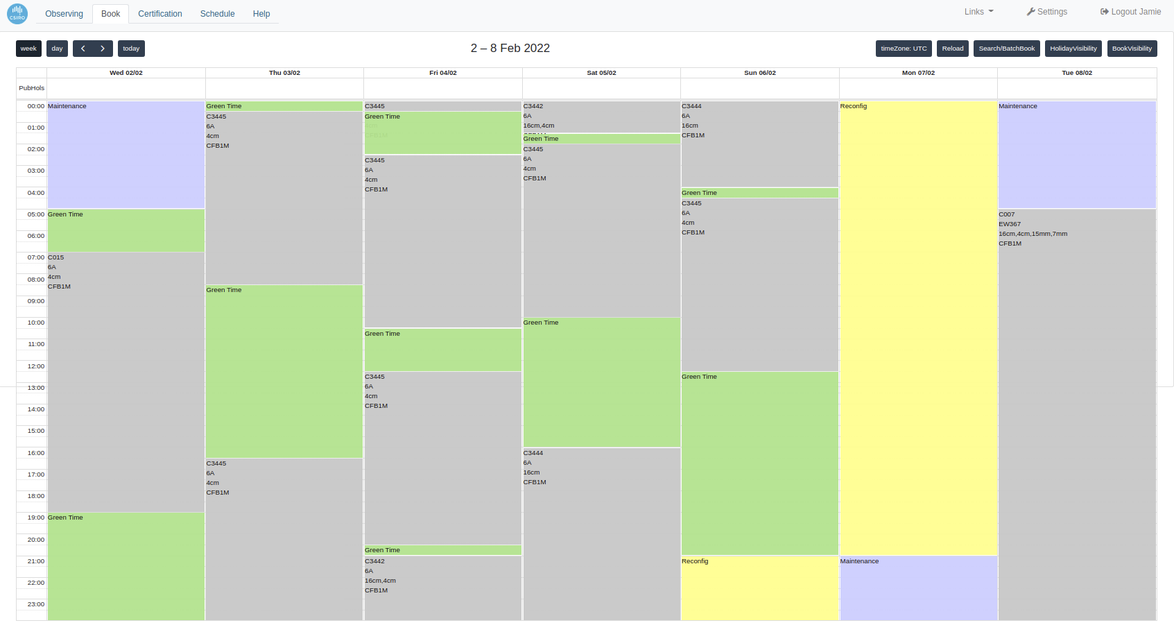
To apply to make an observation remotely, use the “Booking” tab on the ATCA observing PORTAL, which will look something like Figure 2.2. To book for a slot, click on the start time and then drag out a box to the end time of the booking. A booking box will pop up, and you can adjust the start and stop times if you need to.
Remote observers must have their own ATNF UNIX account and remember their password for this account.
To be sure of a successful remote observing session, all observers are required to test their remote observing setup at least a week before their observations.
At a minimum, you will require the following for remote observing:
A computer with SSH software, capable of running a VNC viewer, on a high bandwidth connection,
A telephone near to the computer, that can make calls to, and accept calls from the observatory.
Remote observations will be easier if you also have:
Two or more monitors attached to their computer,
A computer with X-Windows software,
A hands-free speakerphone or headset.
To test your setup, you should contact the duty astronomer and ask to be allowed to login and perform the test. If the test will not disturb current observations, you should follow the instructions on remote observing found in Chapter 3 to ensure that you can monitor and control all the required VNC sessions. If problems are encountered here, and the duty astronomer can't help you resolve them, contact the observatory staff with a description of the problems and ask for advice.