Observations on the ATCA normally consist of a sequence of scans: a scan is a period of observing where the telescope configuration stays the same. A complete observation is made up of a number of scans. Observations typically alternate between scans on the scientifically interesting sources and scans on one or more calibrators. The configuration of the scans and their order are kept in a schedule file.
The main observing task, caobs, reads the schedule file to determine what sources are to be observed, for how long, and in what order. The schedule file also defines the frequencies and correlator setup for each scan and can also be used to make the system automatically execute commands. The ATCA web scheduler is the tool to use to create ATCA schedule files in the CABB era. Schedules made with the old sched program are no longer understood by the CABB version of caobs and thus cannot be used. However, it is possible for the web scheduler to read in old schedules and save them for use with the new system. Please also note that an active ATNF username and password is required to gain access to the web scheduler page.
Generally, users will want to prepare at least two schedule files:
A schedule file for setting up (delay calibration etc.) and flux density calibration. It should include the appropriate flux density calibrator (Section 2.2.4), and if the flux density calibrator cannot be used as a bandpass calibrator, another calibrator with higher flux density that can be used for array setup and bandpass calibration.
A schedule file containing the science program source(s) and gain calibrator(s) (Section 2.2.5).
You may also want to prepare contingency schedule files in case your preferred frequency is seriously affected by interference, or the selected calibrator proves to be resolved.
If your goal is to make a high-quality image of a source that has an angular extent much smaller than the size of the primary beam of the ATCA antennas, then you should observe your source in “snapshots”. The same strategy can be applied if you want to image a small number of sources that are separated in the sky.
Snapshot observations will allow you to obtain a wide range of uv coverage without having to spend all your observing time on source. This is necessary because you will need to obtain calibration data within your time allocation. Generally, a snapshot consists of one or more calibration scans, followed by some integration time on the science target, followed by a gain calibration scan. These snapshots are repeated until your observations are complete.
Snapshot observing is best illustrated with examples.
This is essentially the simplest form of snapshot observing. All you need to do is integrate on the target, and occasionally visit a gain calibrator to ensure that you keep track of any phase changes. A single snapshot might therefore be:
2 minutes integration on a gain calibrator.
40 minutes integration on the target.
2 minutes integration on a gain calibrator.
This set of scans can be repeated as many times as possible within the allocated time.
These scans will give you enough data to properly calibrate the gains during your observing, and the polarisation as well, provided you get more than three snapshots in your allocated time. However you will need to spend some time observing the flux density calibrator (which also works as a bandpass calibrator) at some time during your allocated time.
Imaging several sources is basically the same as imaging a single source, except you have multiple snapshot sets to get through. For each source that you have, you will have an associated nearby gain calibrator. Then, you will have multiple sets that look like:
2 minutes integration on gain calibrator for source 1.
20 minutes integration on the target source 1.
2 minutes integration on gain calibrator for source 1.
During the allocated observing time, each set of scans will be observed multiple times, but it is best to interleave them to ensure you get the widest possible coverage of azimuths and elevations for each set. And once again, you must remember to get some time on the flux density calibrator.
Changing to the higher frequency 7mm band means that you must start doing online pointing correction scans. The basic set of scans is still the same, as in example 2, but now you have to occasionally add in a pointing scan. For example, if your normal scan set takes 20 minutes (e.g. 16 minutes on source, 4 minutes on the gain calibrator), then you could observe this set three times between pointing scans, as it is recommended that you don't use a pointing solution for more than an hour.
If your sources are all within 20° of each other, you may be able to find a single source that can be used as the pointing correction calibrator, and you will only need to do this once per hour.
If your sources are spread around the sky you will need to do a pointing correction for each source. If you are only visiting your sources once per hour, then the pointing correction scan can simply be built into your snapshot set. However if you are looking at each source multiple times per hour, but you want to observe the sources interleaved with each other, you will need to be careful.
Usually, when you do a pointing correction scan, the corrections that are determined
are applied immediately and all subsequent scans (well, those that have
Pointing set to “Offset”) will use those corrections.
This would be a problem if you are observing a source that is more than 20°
away from the location of the most recent pointing scan, even if it was within 20° of the
location of a pointing scan that was done less than an hour ago; such a scan would
use the wrong pointing corrections!
The solution to this is to set Pointing to “Offpnt”
for the scan. In this case, caobs will find the most recent
pointing corrections that are close to the location of the current scan, and use those
corrections for that scan.
In the 3mm band, not only do you need to do pointing corrections every hour, you need to do frequent observations of the paddle. The frequency of your paddle observations is determined by the conditions during your allocated time, and is related somewhat to the required frequency of your gain calibrator observations. That is, if the atmosphere is turbulent, then you may only be able to spend a few minutes away from a gain calibrator. And in such a case, the system temperature may be changing on a similar timescale. It is therefore usually a good idea to include a paddle scan in every snapshot set. Such a set might look like this:
Measurement of the paddle.
2 minutes integration on the gain calibrator.
8 minutes integration on the target source.
Measurement of the paddle.
2 minutes integration on the gain calibrator.
Since the apparent flux density of the sources you are observing will depend on the system temperature measured by the paddle scan, it is very important to ensure that you do the paddle measurement before you observe the sources. It is however not really necessary to ensure the measured amplitudes are accurate before doing a pointing scan.
If the source you will image is bigger than a small fraction of the ATCA primary beam, or the region you want an image for is considerably larger than the primary beam, you will need to use the ATCA's mosaicking functionality.
In interferometry adjacent pointings are not independent and so we can get fundamentally better images by processing the different pointings together. Necessary information about the pointing grid pattern to use for proper Nyquist sampling and the time to be spent on each position to optimise tangential uv coverage can be found in Chapter 21 of the Miriad Users Guide.
For close-packed mosaicking (pointing centres every half-beamwidth), drive times are determined by the acceleration limit of 800°/min². Half the drive time is spent accelerating and half decelerating. For drive times much further than 108′ in azimuth or 27′ in elevation, the drive times are dominated by the slew rate limits of 38°/min in elevation and 19°/min in azimuth. For example, a 16′ drive for a 16cm mosaic will take, depending on the elevation and azimuth of the source, approximately 2.2 seconds. Data taken during the off-source period is blanked in the correlator using a predicted drive time. As drive times can be a significant overhead, care should be taken to not slew the antennas more than necessary.
Mosaicking is less useful if frequency switching is desired, as no frequency changes can occur during the mosaic scan. Since slew times are often much greater than the time it takes for the correlator to switch frequencies, the overheads involved in repeating a mosaic scan for each separate frequency might quickly negate the normal benefits of mosaicking.
Mosaicking mode can also be useful when a large number of nearby sources are to be observed, as observing overheads are reduced. Other applications include holography and source surveys using one dimensional cuts.
When scheduling a mosaic observation, the “snapshot” strategy should be used in order to get calibration data. That is, a point source calibrator should be observed periodically between observations of the mosaic pointings.
If you are mapping a very large, regularly-shaped region at low frequency, where the slew time between each pointing centre is dominated by the maximum speed of the antenna rather than the acceleration/deceleration rate, then you may get a significant reduction in overhead by using on-the-fly mosaicking.
On-the-fly (OTF) mosaicking has a couple of important differences to traditional mosaicking. Most importantly, although the mosaic pattern should be broadly the same – the hexagonal pattern is still the optimal sampling – the order of observations should be such that the telescope scans in a straight line for as long a distance as possible.
During an OTF mosaic, the phase center follows the mosaic points as specified, and the pointing center moves continuously across the pointings. In effect the primary beam of the antennas becomes elongated (to 1.5 beams) in the scanning direction.
To satisfy proper sampling of the sky, the antennas should not move by more than
half a beam per integration cycle, so the spacing of pointings in the mosaic file
should be the same as before. Because caobs assumes
you are scanning in rows or columns, the direction of scanning is inferred from
the next point. At the last point of a row or column the previous direction is
maintained to complete the scan. One extra point, marked with the name
“TURN”, needs
to be specified at the start of the next row/column, to allow the antennas
to change direction and scan at the correct speed again.
The primary advantage of OTF mosaicking over regular mosaicking is its speed in covering a large area of sky, making it possible to get good uv coverage of a large field in a single observing run. It will not usually provide any better sensitivity than a carefully-crafted regular mosaic.
Although OTF mosaicking is most useful at low frequencies where the slew time between mosaicking points is a significant fraction of the total integration time, this mode could also be used for mm observations by using bin mode and moving the antennas by e.g., 16 beams in a single integration with 32 time bins. The Miriad program atlod will need some work to properly record the phase center and pointing center in this case (ie. such a mode is not currently supported, but may be if demand for it is high).
Mosaic observations use a standard schedule file and an additional file,
called the mosaic file,
which lists the positions of the mosaic field centres.
Up to 2048 fields can be specified in a single file.
This mosaic file must consist of one line per pointing centre in the
mosaic pattern. Lines beginning with the “#” character
are ignored and can be used for comments.
The general mosaic file format is:
# Comments  .... ignored by the software
#
d(RA)  d(DEC)  INT  $FIELD_1
d(RA)  d(DEC)  INT  $FIELD_2
d(RA)  d(DEC)  INT  $FIELD_3
d(RA)  d(DEC)  INT  $FIELD_4
The items in each line are:
“
d(RA)” the offset Right Ascension of the pointing centre, in “degrees of polar rotation”, from the reference position. For example,d(RA) = +15.00will move +1 hr in RA at all declinations.“
d(DEC)” the offset declination of the pointing centre, in degrees, from the reference position. e.g.d(DEC) = +1.000will move the pointing centre one degree north.“
INT” the integral number of integration cycles to spend on each pointing centre.“
$FIELD_n” the name of the field. The “$” symbol is a prefix to the field name, and indicates that scans will follow in the order as they are listed in the mosaic file. The field name must be different for each pointing centre and must have 9 or fewer characters (naturally, “$” can not be used as the first character of the field name). Note: If you wish to use the “mosaic” option in the Miriad task uvsplit (to keep the mosaic pointings together in one uv data file), the field name strings should differ by only the “_n” part of the name, where “n” is an integer. The field name given within the mosaic file does not need to match the source name given in the schedule file.
This file should be named “mosnam.mos”. The
“.mos” suffix is required, or
caobs will not find the file. The
“mosnam” part of the name
must match the source name given in the
schedule file.
To include a mosaic in a schedule file, insert a scan and set:
“
Source” to the name of the mosaic file, excluding the “.mos” extension, i.e. “mosnam”.“
ScanType” to “Mosaic”“
RA” and “Dec” to the reference position for the mosaic, i.e. the position that all the mosaic field centres are offset from. Check this carefully. Then check it again. Although the reference position is usually included as a comment in the mosaic file, caobs reads only the coordinate offsets from the mosaic file. Therefore, if the reference position is set incorrectly in the schedule file, caobs will not warn you, and your observations will fail.
All other scan settings have their usual effect, including the
“Pointing” mode, and the observing
frequencies.
The mosaic file must be placed
in the /atca/mosaic directory on xbones so
that caobs can locate it during the
observations. The mosaic file name must be completely in
lowercase letters, even if the corresponding source name in
the schedule has uppercase letters;
caobs will report that the mosaic file
could not be found unless it has an all-lowercase file name.
The “.mos” suffix is required, or
caobs will not find the file.
The file can be copied into position manually, but there is also a web interface that will ensure your mosaic files are put in the correct location.
The time specified in the “ScanLength” field
in the schedule file will determine how many times the mosaic
is looped through in a single scan. caobs
calculates this by dividing the “ScanLength”
time by the total length of the mosaic and rounding this to
the nearest integer; this will be the number of times the
mosaic is repeated during this scan. The mosaic is always observed at least
once, regardless of the “ScanLength”.
It should be noted, in particular for mosaic files containing sources spread over a range of RAs, that if caobs encounters a source in that has set (or not risen), it will skip to the next scan in the schedule file, not to the next source in the mosaic file.
The following example shows a mosaic file specifying a four pointing centre pattern on a 0.25° grid. Note that the RA offsets are coordinate increments not sky distances.
Mosaic file: mymap.mos |
# mymap.mos by P. Smith
| |||
# A four pointing centre mosaic
| ||||
# Ref. Position = 05:21:33, -65:56:41
| ||||
0.0000 | 0.000 | 2 | $mymap_1 | |
0.6133 | 0.000 | 2 | $mymap_2 | |
0.6133 | -0.250 | 2 | $mymap_3 | |
0.0000 | -0.250 | 2 | $mymap_4 | |
The scan in the corresponding schedule file might have the parameters:
| Scheduler fields: | Source: | mymap | Observer: | Smith | Project: | C555 |
RA: | 05:21:33 | |||||
Dec: | -65:56:41 | |||||
Epoch: | J2000 | |||||
ScanLength: | 00:30:00 | |||||
ScanType: | Mosaic | |||||
Pointing: | Global |
With these settings, and with the default integration time of 10
seconds, the four pointing centres will be observed every 80 seconds.
Since the “ScanLength” is 30 minutes, the mosaic will be repeated
23 times (22.5 is rounded up), but if the “ScanLength” was 29.5
minutes, the mosaic would only be repeated 22 times (22.125 is rounded
down).
Here is a 3x3 pointing grid around a source; we use 1934-638, but the same offsets could be used for any source.
0.0000    0.00    2  $@1934-on C
-0.1812  -0.16    1  $TURN-10
-0.1812  -0.08    1  $1934-11
-0.1812   0.00    1  $1934-12
-0.1812   0.08    1  $1934-13
0.0000    0.16    1  $TURN-24
0.0000    0.08    1  $1934-23
0.0000    0.00    1  $1934-22
0.0000   -0.08    1  $1934-21
0.1812   -0.16    1  $TURN-30
0.1812   -0.08    1  $1934-31
0.1812    0.00    1  $1934-32
0.1812    0.08    1  $1934-33
Note that you can specify a non-scanning position in an OTF mosaic file by starting
the field name with a “@”, like the 2 cycle calibration on
“1934-on” above. Also
note the fields marked with “TURN” - these are the extra
points required at the
start of each scanning row/column to give the antennas time to get to the correct position
and scanning speed. They should be discarded when processing the data.
Note also that all other pointing centres in the OTF mosaic file are only observed for 1 cycle. This cannot be changed, since the antenna will be moving while it observes each pointing.
To use
the OTF mosaic mode, specify a scantype of
“OTFMos” in the web scheduler and
put a mosaic file like the one above in “/atca/mosaic” on
xbones.
The Miriad tasks mosgen and atmos may be useful when you are preparing your mosaic file.
If you need to map a region of known size around a known sky location, you will want to use mosgen. It will overlap each pointing correctly with hexagonal tiling, and will ensure that the pointings are observed with minimal overhead.
If you have a number of specific locations you want to observe, you will want to use atmos, as it will ensure that the offsets are correct and that the route between the pointings is optimised (the “travelling salesman” problem).
We do not recommend that you manually calculate the offset positions for your mosaic. An error in calculating the offsets will likely ruin your observations. Such an error is easily avoidable by using the Miriad tasks.
How large the mapping region is will determine whether you can image using standard snapshot observations, or if you will need to use mosaicking. In either case, the imaging strategy is no different to that of a continuum observation, but you may need more frequent calibration to ensure you get a sufficient signal to noise ratio for your lines; CABB's extra bandwidth doesn't help you observe a single line at known redshift!
If you're looking for your spectral line in one of the CABB continuum IFs, one of the most important things to consider is where the line to be observed will fall within the bandpass, ie. which channel(s) it will appear in. There are several channels in the CABB continuum IFs that are always flagged, and several more that are often contaminated with self-generated interference, and these should be avoided when observing spectral lines.
The CABB correlator always flags the centre continuum channel and each of the quarter-band channels. If you select a CABB mode that provides 1 MHz continuum channels, the flagged channels will be 513, 1025 and 1537. For CABB modes that provide 64 MHz continuum channels, the flagged channels will be 9, 17 and 25. You should avoid making the central CABB continuum frequency the same as the expected frequency of the line.
Self-generated interference will likely be present in the 1 MHz continuum channels 129, 157, 257, 641, 769, 1153, 1177, 1281, 1409, 1793 and 1921. All these channels can be easily flagged with the online correlator software (and they routinely are) and the interference does not leak into the adjacent channels.
If you are using the CABB zoom bands to detect your spectral line, you should again avoid using one of the continuum channels listed above, especially the quarter- and half-band channels. The zoom bands derived from those channels will usually have a very large spike at the centre of the zoom, and this spike may leak into adjacent channels since the zoom channels are not perfectly square. However, since the zooms come from the interleaved channels, the zoom channel number is derived from the continuum channel number by multiplying by 2 and subtracting 1. For example, channel 17 in the 64 MHz continuum band is actually zoom channel .
It is important to note that ATCA is not able to Doppler track. You will need to ask for enough frequency coverage to ensure that your line will not drift out of the band due to observatory velocity changes.
Calibration of spectral-line observations is done with the same “snapshot” strategy that was described in Section 2.3.2. It is important to note however that the calibration itself is slightly different. Because accurate measurements of a spectral line requires good bandpass characterisation, but in general you are dealing with much smaller bandwidths than for continuum observations, you will need to observe calibrators with higher flux densities, observe the calibrators for longer, or observe the calibrators more often in order to get a sufficient signal-to-noise ratio.
There are many restrictions on the frequencies that can be observed with the CABB system. The most basic restriction is that only two 2048 MHz IFs can be observed simultaneously. All of the additional zoom bands must lie within these IFs, so they do not count as “extra” bandwidth. You can only specify the central continuum frequencies to MHz precision.
If you want to use the entire array for a single band, then there are band-specific restrictions on the frequencies that can be observed.
In the 16cm band, the central frequency of each continuum IF must obey MHz.
In the 4cm band, the central frequency of each continuum IF must obey MHz.
In each of the mm bands, the centre frequencies of the two continuum IFs cannot be separated by more than 6000 MHz, ie. MHz.
In the 15mm band, the central frequency of each continuum IF must obey MHz.
In the 7mm band, the central frequency of each continuum IF must obey MHz.
In addition, the IF centre frequencies must both be below 40673 MHz, or both be above 41227 MHz.
In the 3mm band, the central frequency of each continuum IF must obey MHz.
If you don't need all the baselines in the same band, it is possible to split the array up
so you can observe in two bands simultaneously. For each of the two CABB
continuum IFs you can select a set of antennas to use with the
caobs command “set band1_antennas”.
In this way you can specify a frequency in IF1 that is in a different band
to the frequency specified in IF2. The antennas specified in the
“band1_antennas” would use the IF1
band, while the rest of the array would use the IF2 band.
The primary restriction in this mode is the central site oscillator. Since there is only one central site oscillator that feeds the entire array's L86 modules, if you want to observe in more than one mm band simultaneously, both the frequencies must be observable with the same central site frequency.
You cannot observe in both the 15mm and 3mm bands simultaneously.
Observing in the 15mm and 7mm bands simultaneously is possible if the 15mm central continuum frequency obeys MHz, and the 7mm central frequency obeys either MHz, or MHz.
Observing in the 7mm and 3mm bands simultaneously is possible if the 7mm central continuum frequency obeys either MHz, or MHz, and the 3mm central frequency obeys either MHz, or MHz.
Since neither the 16cm or 4cm bands need the central site synthesiser, there are no special frequency restrictions when one of the simultaneous bands is 16cm or 4cm.
It isn't possible with CABB to observe more than 4096 MHz of bandwidth simultaneously, but it is possible to quickly switch between frequencies within a single band, and also to swap between different bands with only a moderate loss of simultaneity.
If you want to change frequencies, you will need to start a new scan in the schedule. This restriction makes it impossible to change frequencies within a mosaic. Whenever you change scans you will experience two integration cycles of overhead, and if you are changing frequencies within a band, this is the only applicable overhead. For example, if you changed your central continuum frequencies from 5500 & 7500 MHz to 6500 & 8500 MHz, you will only need to incur two cycles of overhead as the scan is changed.
There is also no extra overhead when changing the zoom band configuration, which is simply viewed as a change of frequency within the same band.
If you are changing bands, you will likely incur more overhead. In this case, the turret on the antennas will need to rotate to put the new receiver at the right position, and if you are changing to or from the 7mm band the mm receiver package will need to be moved using the translator as well. Turret rotations will usually add only a few cycles of overhead at most, since the turret can be rotating during the normal two cycle overhead that occurs at every change of cycle. Translating the receiver to go to or from the 7mm band takes much longer: between 2 and 3 minutes.
When you change bands you may also have to refocus the antenna by moving the subreflector. When going to or from the 4cm band, all antennas need to be refocused, and this takes approximately 90 seconds. When going to or from the 3mm band, antenna CA01 needs to be refocused, and will take approximately 40 seconds.
WARNING: Movement of the turret does produce wear on the bearing, and it would be extremely difficult to replace it should it fail. We therefore ask that observers not change bands more than once every 15 minutes.
To schedule an observation of a major planetary object, simply put
its name in the “Source” field of a scan. During the observations,
caobs will interpret this name and calculate where the planet, Sun
or Moon is and point the array towards it.
The scheduler will not automatically calculate where the planet will be during
the scheduling process, unless you enter the appropriate date and LST or UTC and then
click on the “Listing” tab. At this point, the
scheduler will determine the planet's position and fill the “RA” and
“Dec” fields. Alternatively, you could use
the Miriad task planets.
It is useful to note again that the “RA” and
“Dec” fields are ignored by caobs
when the source name is recognised as a planet, the Sun or the Moon, as
caobs will compute the appropriate position for the body in
real time. There is no reason therefore to prefer absolute time scheduling when
observing planets.
Solar system objects differ from most astronomical sources in that the proper motions are large enough that the object position may change in the course of an observation. caobs has the ability to phase track an object with a non-sidereal rate, and command the antennas to correctly track it as well. If the object moves across the sky too quickly however, the antenna speed limits may prevent you from tracking the object.
For minor bodies, caobs cannot compute a position, so the correct
position must be provided by the user. The scheduler
treats source names beginning with the @ symbol (eg. a source name of
@hbopp) as pointing to an external ephemeris file (eg. a file
$ATCA_EPHEM:hbopp.eph).
Ephemerides for minor solar system bodies can be computed before scheduling using JPL's Horizons on-line system. Only the telnet (terminal-based) access method is described here, but there is also a web-interface method available from the web page that is self-explanatory.
Horizons asks the user a series of questions. To generate an ephemeris file for ATCA observations:
telnet horizons.jpl.nasa.gov 6775
First select an object by giving the source name (followed by a semi-colon for minor bodies) or by source number.
In response to prompts, select “
Ephemeris”, then “Observe”, then “Geo” to select geocentric RA/Dec ephemerides.Give the start time of interest, in UTC, in the format suggested by the prompt. At the next prompt give the end time, and then the time increment; typically 1 minute (“
1m”) will give you the best chance to accurately track the object. The scheduler uses simple linear interpolation of the ephemeris values. The ephemeris supplied to the scheduler must start at least two time increments before the scheduled start time, and must extend beyond its end time.Accept “
default output”, and at the “Select table quantities” prompt, enter “1,20” to get RA, Dec, distance and velocity of the object.Horizons will then display the ephemeris in the terminal. To get it to email the ephemeris, press “
q” and the main menu will be displayed again. Then select “[M]ail” and enter the email address to send the ephemeris to.To log out of Horizons, press “
Ctrl-D” (the terminal hangup signal).
The ephemeris file produced by Horizons needs to be massaged into the format that the scheduler requires. This is best achieved with the ephformat command available on xbones.
First, copy the ephemeris from the email sent by Horizons into a plain text file on xbones.
Run the command ephformat with no arguments.
At the first prompt, give the name of the text file with the Horizons ephemeris (including file extension). At the second prompt, give a short descriptive name for the output ephemeris file (excluding any file extension). ephformat will then write out the appropriate ephemeris file to “
$ATCA_EPHEM:file.eph” where “file” is the name entered at the second prompt.
To use the ephemeris you just created in the schedule, enter the name of the
ephemeris (the “file” name described in the last
dot point above), preceded by the “@” symbol, into
the “Source” field of the web scheduler.
There is a limit to how far the antennas can slew in azimuth. The limit arises because of all the cabling inside the antenna which passes up the centre of the structure to the receiving and cryogenic equipment in the vertex room. There is a limit to how far these cables can wrap around in either direction (similar to the head of an owl).
The wrap limits for the ATCA antennas are CCW=152.5° and CW=327.5° as shown in Figure 2.1.
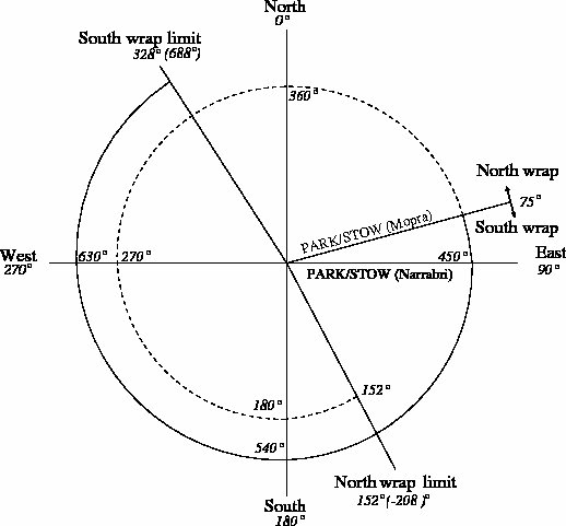
It is a good idea to check what wrap the telescope is in at the start of your observations, as “unwrapping” can take up to 10 minutes. To determine the wrap you are in, consult MoniCA or atdrivemon. MoniCA shows the wrap explicitly, on the “ATCA Summary” page. atdrivemon shows the azimuth using the ATCA convention — while in the South wrap azimuths are expressed as positive angles, and negative angles in the North wrap.
The CABB web scheduler is used to prepare schedule files. The web scheduler checks the schedule for completeness and, where possible, checks choices such as observing frequency for hardware compatibility. Drive times, and source azimuths and elevations can also be computed to enable you to estimate overheads and observability.
Three steps are involved in using the web scheduler:
A new scan is added to the schedule.
The details of the scan are changed as desired.
When all the scans have been defined, the entire schedule is written to file.
When constructing a schedule, consider:
Is the sequence of sources sensible, and how much time is expended on slewing?
Does the schedule contain all the sources, and at the appropriate frequencies and bandwidths?
The web scheduler can produce a listing to help answer these questions.
It is a good idea to study these listings very
carefully before observing commences. The scheduler considers drive times:
all coordinate entries are automatically followed by a calculation of the
azimuth and elevation of the source, as well as the drive time from
the previous source, using the entered value for LST. When making
a schedule file, the integration times are specified
for each source (and calibrator source). Note that,
except in the case of mosaic schedules and Dwell scan types,
these integration times
include drive times, so the specified time must be somewhat longer
than the amount of integration on source required. This is
particularly important for gain calibrators, when the drive time
(up to a minute or so) may be comparable to the integration time
(one to three minutes). Alternatively, the ScanType field can
be set to Dwell to ensure a source or calibrator
is tracked for the specified scan duration.
The schedule file submitted to caobs (the online Compact Array control
task) need have no specific start time. Rather, the schedule file asks
caobs to start the first scan as soon as possible. The sequence of
scans will be exactly as specified in the schedule file. However, when
using the web scheduler, the calculation of azimuths, elevations and drive times
is possible only if the starting sidereal time is known (at least
approximately). The sidereal time for the first scan in the schedule
can be set in the web scheduler by giving the time in the Time field,
and setting TimeCode to LST. Alternatively, the starting UT
may be specified by setting TimeCode to UT, and by setting
the Date to the appropriate start date by clicking on it and using
the calendar that appears. Note that when viewing any scan other than the
first in the schedule, the fields Time, TimeCode and
Date all become read-only.
The environment flag can be used to instruct the online software to remember certain settings, such as attenuators, and to recall them whenever a scan with the same environment flag is encountered. However, this is generally not required, as the online software will remember user settings, and recall them when the same conditions are encountered again. There are at least 128 slots for user settings, so for a normal schedule, the environment flag will probably not need to be used.
See Appendix F for a complete guide to all the functionality available in the web scheduler.
Yes! In this section a simple continuum schedule file is constructed. It will contain three sources: a program source and two calibration sources. The following observing sequence will be specified:
Setup calibrator (0537-441, a catalogued source) for 5 minutes,
Program source (R.A. 05:21:35.5, Dec. -21:24:27.1 (J2000)) for 30 mins,
A gain calibrator for 5 minutes.
These sources will be observed at the standard 4cm band frequencies of 5500/9000 MHz. To create this schedule file, perform the following steps (instructions are given in bold, and the results of the instruction, or important caveats, and described below it):
- Navigate to the CABB web scheduler in a web browser.
The first screen is displayed.
-
Change the
Sourcefield totest, theRAfield to05:21:35.5and theDecfield to-21:24:27.1. The delimiter for coordinates must be a colon, and the default
EpochofJ2000should only be changed if necessary.-
Change
ScanLengthto 00:30:00 and change theScanTypetoDwell. This ensures that 30 minutes are spent on source, regardless of slewing times.
-
Ensure
Pointingis set toGlobal. Offset pointing is not required for low-frequency observations.
-
Change the
Observerfield toWild, theProjectcode toC123. These fields should be set in the first source - they will propagate to the other sources as they are added.
-
Change the
Timefield to02:00:00, and theTimeCodefield toLST. This indicates that the schedule will be started at an approximate LST of 2h.
-
Click the
Freq1 Setupbar. This brings up the frequency selection fields.
-
Enter
5500in theContinuumfrequency box, and keep theChn. BWselection box to1MHz. The velocity resolution should be calculated to be 55 km/s, and the velocity range will be 111632 km/s.
-
Click the
Freq2 Setupbar. This brings up the frequency selection fields.
-
Enter
9000in theContinuumfrequency box, and keep theChn. BWselection box to1MHz. The velocity resolution should be calculated to be 33 km/s, and the velocity range will be 68219 km/s.
-
Click the
Scan Parametersbar. This brings up the scan details.
-
Click the
Search Calbutton. This presents a list of nearby calibrators to the right of the scan details, sorted by distance to the source. The closest source to the program source with a moderate flux density (> 1 Jy) is shown to be 0454-234, at a distance of 6.02°.
-
Click on the
0454-234button. The details for this source are displayed from the calibrator database below the source list. This source is a suitable gain calibrator as it has a decent flux density, has a defect less than 0.1% and a closure phase less than 0.3%.
-
Click on the
0454-234button again. Clicking on the button twice (without clicking another source button between clicks) inserts this source into the schedule above the currently selected source.
-
Select source 1, and change the
ScanLengthfield to 00:05:00. -
To copy this source to the end of the schedule, click on the
Editmenu and selectCopy, then select thetestsource, click onEditand selectPaste. The schedule should now have three sources (in order): 0454-234, test, 0454-234. The first source needs to be changed to 0537-441.
-
Select source 1
,
Change the
Sourcefield to 0537-441 and pressTAB. The scheduler will automatically put the source coordinates for this known calibrator in the
RAandDecfields.-
Click on the
Filemenu and selectSave As. The
Schedule file selectorwindow will appear.-
The schedule will be called c123_test.sch, so enter this into the
Filterbox to ensure that there is not already a schedule with this name. If there is another schedule with the desired name, consider changing it.
-
Enter
c123_test.schinto theSchedulebox and press theSavebutton. The file selection window will disappear, and the name of the schedule should now appear at the top of the window.
To produce a listing of the schedule, in order to check that the
schedule proceeds as expected, click on the Listing tab.
Yes! This example adds to the example from the previous section; ensure that the schedule created in the previous section is in the scheduler before continuing.
Now the aim is to observe 1 zoom band in each IF, each covering at least 70 km/s. The galaxy “test” is actually at an LSR recessional velocity of 25000 km/s, and these observations will look for CH3OH methanol and HC3N cyanoacetylene lines.
To create a schedule that can perform suitable observations for this situation, follow the steps:
- Select the first scan in the schedule.
This should be 0537-441.
-
Select the
Global changemenu item from theToolsmenu before changing theDateof this scan to 30/11/2014. The date that the observation will be performed is required to ensure that the observatory velocity is computed correctly.
-
Hit the
Global Applybutton. The date will now change for all the sources in the schedule.
-
Select the
Advanced viewmenu item from theToolsmenu. You should now see many more input fields.
-
Select the “
test” source in the schedule, then enter “25000” into theCatVelfield, and press TAB. The entry in the
CatVelfield should now read “25000 lsr radio” as the default frame is LSR, in the radio convention.-
Click the
Freq1 5500MHzbar. This brings up the IF1 frequency selection fields.
-
Click the topmost
Velobutton. This brings up the velocity calculator.
-
Select the
CH3OHline from theSpectral Linedropdown box. The rest frequency of this line (6668.518) appears in the
Rest Frequencybox below. TheSky Frequencywill be updated to 6112.092 MHz, and the zoom band frequency will be calculated as the nearest half-MHz, in this case as6112MHz.-
Click the
Applybutton in the velocity calculator. The velocity calculator will disappear and information will be inserted into the first zoom band. In this case, the
6112MHz frequency translates into the channel3273. The velocity resolution is given as 0.024 km/s, and the velocity range is listed as 49 km/s.-
Select the zoom band width to be
2from the width drop box. The velocity range now increases to 73.6 km/s.
-
Click the
Freq2 9000MHzbar. This brings up the IF2 frequency selection fields.
-
Click the topmost
Velobutton. This brings up the velocity calculator as before.
-
Select the
HC3Nline from theSpectral Linedropdown box. The rest frequency of this line (9098.332) appears in the
Rest Frequencybox below, and theSky Frequencywill be updated to 8339.161 MHz. The zoom band frequency will be calculated to be8339MHz.-
Click the
Applybutton in the velocity calculator. The velocity calculator will disappear and information will be inserted into the first zoom band. In this case, the
8339MHz frequency translates into the channel727. The velocity resolution is given as 0.018 km/s, and the velocity range is listed as 36 km/s.-
Select the zoom band width to be
3from the width drop box. The velocity range now increases to 71.9 km/s, comparable to the width provided for the IF1 zoom band.
-
Click the
Scan Parametersbar. This brings up the scan details.
-
Select the
Master1option from theFreqConfigdropdown box. This signifies that the frequency configuration, including the zoom modes, from this scan, should be defined as the master configuration.
-
Select the
0537-441source from the schedule, then elect theSlave-1option from theFreqConfigdropdown box. Now this scan will exactly mirror the frequency and zoom mode configuration from the
testscan, even if the configuration of thetestscan is changed. When a scan is set as a slave scan, theFreqpanels will display a message describing which frequency and scan it is slaved to.-
Select the
0454-234source from the schedule, then select theSlave-1option from theFreqConfigdropdown box. Now this scan will exactly mirror the frequency and zoom mode configuration from the
testscan.
At this point, the schedule would correctly describe a zoom mode observation.