Australia Telescope National Facility

Only Miriad can read in raw CABB RPFITS files, with the atlod task. However, CASA can use its importmiriad task to take the output of atlod and convert it into the more commonly-used MeasurementSet (MS) format.

Both packages are capable of flagging CABB data, but generally speaking, the Miriad routines (such as uvflag, blflag and pgflag) are easier to drive, and give excellent results.

Both packages can do a full calibration of the data, including flux density calibration (the latest models for 1934-638 are in CASA), and polarisation calibration. The only significant difference is that CASA gives you much more control about where different effects are considered in the calibration tables; both will give excellent calibration however.

Imaging is where the Miriad and CASA packages differ greatly. Miriad allows you to make images over wide bandwidths, and does a good job of making spectral cubes as well. It also handles making mosaicked images, but lacks the ability to do mosaicking over a wide bandwidth.

To do that properly, you will need to turn to CASA, which is also able to handle doing multiscale cleaning, and does uv-based cleaning instead of Miriad's image-based cleaning.

For a simpler but more capable imager, you may also want to consider using wsclean, which supports most of what CASA does, but is very easy to drive.

Miriad development is mostly static, but code to fix bugs may be introduced at any time. It is therefore important that before beginning your data reduction you obtain the very latest Miriad distribution.

To get the latest Miriad distribution, please follow the instructions in the install guide. Once you have it installed on your computer, it is easy to keep up-to-date. If you installed the binary version of Miriad (which is highly recommended), you can receive updates by running

$ mirsync -u usr123

where usr123 should be replaced with your ATNF UNIX user name. If you installed from source, then you can use the mirimport command to get updates, after which you will need to recompile Miriad.

It is also important to report any problems you may have with your reduction to the Miriad maintenance team so that any issues can be resolved. If you experience any problems, please use the mirbug routine, or send an email describing your problem to <miriad@atnf.csiro.au>. If you don't think your problem is related to a bug, but you need advice on how best to proceed with your reduction, please ask for help using the ATCA Forum. ATCA and ATNF staff routinely check the forum and answer questions from the community, making the forum a good place to start to look for answers as well.

To load CABB data, you will use the atlod task. This section discusses how to use this command most effectively.

For CABB data, a number of channels are affected by self-generated interference from the 640 MHz CABB clock, and the birdie option flags these channels during load. It also flags out 4.9% of channels on each band edge (which works out to be 100 channels for CABB's 2049 channel spectra) and, for 20/13cm data taken before 2010-Aug-17, the unusable parts of the spectrum in the old, separate 20cm and 13cm bands. These unusable parts are due to the fact that these receivers did not respond to all frequencies across the 2 GHz bandwidth of CABB. This option still works for pre-CABB data as expected.

If you wish to change the number of edge channels that are flagged by the birdie option, use the edge parameter in atlod. By default it is set to 9.8 (per cent), which works out to 200 channels for a 2049 channel spectrum. These flagged channels are split evenly to the top and bottom of the spectrum, so if you wanted to flag only 32 channels on each band edge for example, you should specify edge=3.1.

The rfiflag option can be used now to automatically flag out frequency bands that are known to be heavily affected by RFI. This option is most useful in the 16cm band, where the ATCA receivers are routinely affected by strong RFI. It is completely safe to use at any band however, and should be included in the default list of options when you use atlod. The file it uses to determine the flagging it performs can be customised to include extra flagging (or less flagging) if so desired. By default, this file (called rfiflag.txt) can be found in the directory cat in the Miriad tree. To customise it, copy it to your reduction directory, insert or remove more frequency ranges to flag, and then load your data with atlod.

Note that the rfiflag option will have no effect if the birdie option is not also specified.

Another useful atlod option is xycorr. This corrects the measured XY phase of the ATCA, and can be safely included at all bands for CABB data.

By default, CABB records the autocorrelations from each of the antenna that are being used, which may not be useful if all you are interested in is the cross-correlations required to make an image. Having the autocorrelations present during the reduction does no harm to any of the Miriad routines, but may become confusing and/or annoying when trying to examine the data. You can make atlod discard these data by using the noauto option.

The other atlod options are usually band-dependent. Examples of atlod use are given below for all ATCA bands.

For higher frequency data, the atfix routine may be required to apply corrections to the antenna positions and system temperature measurements.

During a baseline reconfiguration at the ATCA, staff perform a baseline calibration (to determine precisely where each antenna is with respect to each other) at 5 GHz and 17 GHz. During normal observing, the solution determined at 5 GHz is applied on-line, and is usually very good. However, for mm data, you may wish to use more precise antenna positions obtained from the 17 GHz baseline calibration. This may aid in phase referencing experiments.

The atfix routine can “fix” the positions of the ATCA antennas based on the solution file that is made available by the ATCA staff on the baseline solutions page. The high-frequency baseline solutions are not routinely computed for each reconfiguration, so if you'd like to have one, please contact ATCA staff with your request.

The task atfix is also highly recommended for the reduction of 3mm data. During an observation at 3mm, the system temperature is determined using the paddle during a so-called “paddle scan”. These scans are usually tens of minutes apart, during which time the system temperature recorded by the correlator does not change. To make Miriad interpolate the system temperature between the paddle scans, use atfix with default parameters, or with tsyscal=interpolate explictly set.

Task:   atfix
vis      = 3mm_data.uv
select   =
out      = 3mm_data_fixed.uv
dantpos  = 
tsyscal  =
options  =
array    =

After loading the data into a Miriad dataset, it is usually most convenient to split this into many datasets, each containing an individual source at a single central frequency. This is done using the uvsplit task.

At its simplest, it can be run with only the vis parameter set to the parent dataset, but it is also very easy to use the select parameter here to discard data that was affected by antenna shadowing:

Task:   uvsplit
vis      = c007.uv
select   = -shadow(22.5)
options  =
maxwidth =

The select keyword can also be used to split out only certain sources, or to effectively flag out certain antenna. Read about the select keyword in the Miriad manual.

There are two options that are useful here. Specify the mosaic option if you are splitting a dataset that contains a mosaic observation, and specify the clobber option if you want to overwrite any previously split-out datasets in the current directory.

The maxwidth parameter is new to the CABB era, and allows you to break up the 2 GHz CABB bandwidth into smaller chunks. This will be most useful at lower frequencies where 2 GHz represents a large fractional bandwidth. At such frequencies, calibration and imaging is far more challenging than at higher frequencies. The bandwidth specified here should be specified in GHz. For example, to mimic the maximum bandwidth available from the old correlator, you could specify maxwidth=0.128 here. Recent experience shows however that excellent calibration can be obtained using the entire 2 GHz band simultaneously, even in the 16cm band. Splitting up the band at this point then is only recommended for those who have an actual need to do so.

In most cases, if the birdie and rfiflag options are given to atlod, the data will be mostly free from the most destructive RFI at this point. However, you should always examine your data with the uvplt and uvspec tasks to make sure.

Using uvplt, examining amplitude and phase versus time is a good way to find time ranges that have been affected by RFI. Ensure that you specify options=nofqav to prevent uvplt from averaging your data over frequency before plotting. Any RFI present in your observations may be restricted to only a few channels, and these channels can be identified by using uvspec.

To flag this data, you can use the following tasks.

One trap that you may find is that if you are observing at 3mm and some other band in the same run, and you elected to keep CA06 tracking for the 3mm observations, the data from CA06 will not automatically be flagged. This is because CA06 has almost all the systems required for 3mm observing (save for the electronics), and so the antenna really is “on source” according to the telescope. You should use uvflag to flag out CA06 data in this case.

Automatic flagging with pgflag can be very effective if it is done in the right way. It is most useful for continuum observations in any band, and for spectral line observations when the line is not detectable in a single integration. If your spectral line is bright enough to be detected in a single integration, then the flagging routine will likely identify it as RFI.

The pgflag task accepts a number of parameters that control the automatic flagging process. Craig Anderson identified, through trial and error, a recipe that works quite well for 16cm data; this recipe is described in an ATCA Forum post Craig started. We describe this recipe here as well, and we recommend this recipe for data in any band.

This flagging recipe uses the concept that the polarisation properties of interference are quite different to that of the signals we're interested in. For the most part, the radio sky is free of discrete sources of circular polarisation, and thus most measurements of Stokes V from our interferometer should be thermal noise only. This assumption holds over all frequencies as well. So if we see a large deviation from thermal noise in Stokes V, and this deviation is confined to a narrow range of frequencies, the most likely culprit is RFI. The first step of the flagging recipe then is to look for such signals in Stokes V and flag all the visibilities over the frequencies and times they are seen. To do this with pgflag:

$ pgflag stokes=i,q,u,v flagpar=8,5,5,3,6,3 "command=<b"

This flagging can be done on each individual source after it has been split out. Of course, because the output of the interferometer should not vary for Stokes V regardless of the field being observed, you can also flag a single IF all together. That is, you can take a dataset output by uvsplit with options=nosource and flag it directly without further splitting it into individual sources. You can also do the flagging before and after calibration. Indeed, you may have success in doing an initial round of Stokes V flagging before trying to mfcal the bandpass calibrator, and another round of flagging with the same command after calibration.

As an illustration, Figure 4.1 and Figure 4.2 show what pgflag will display when told to show Stokes V from a dataset centred at 2100 MHz (a typical 16cm dataset) with fourteen scans on nine different sources, obtained in October 2015. Channel number is shown along the horizontal access, and as the 16cm band is presented to the correlator as a lower sideband, higher channel numbers correspond to lower frequencies. The time of the observation increases along the vertical axis towards the top of the image and the amplitude of each channel is represented as a grey scale which is outlined in purple toward the right of the image. Flagged regions are shown as completely black. Figure 4.1 shows a 60m baseline and Figure 4.2 shows a 4469m baseline. The only flagging done to this dataset is at the edges to remove the roll-offs, which removes 10.5% of the data on each baseline, and the data are uncalibrated. These two figures clearly show how much more sensitive short baselines are to RFI than long baselines.

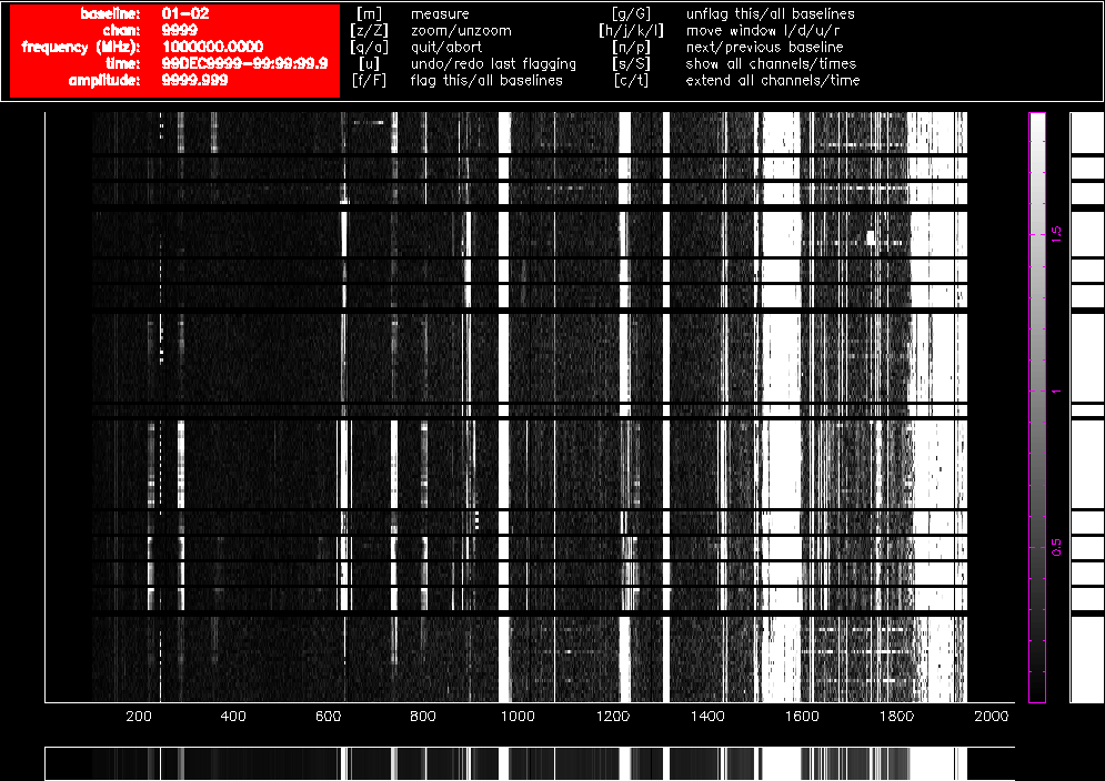
Figure 4.1. A pgflag display showing Stokes V data on a short baseline in a 16cm dataset before flagging.

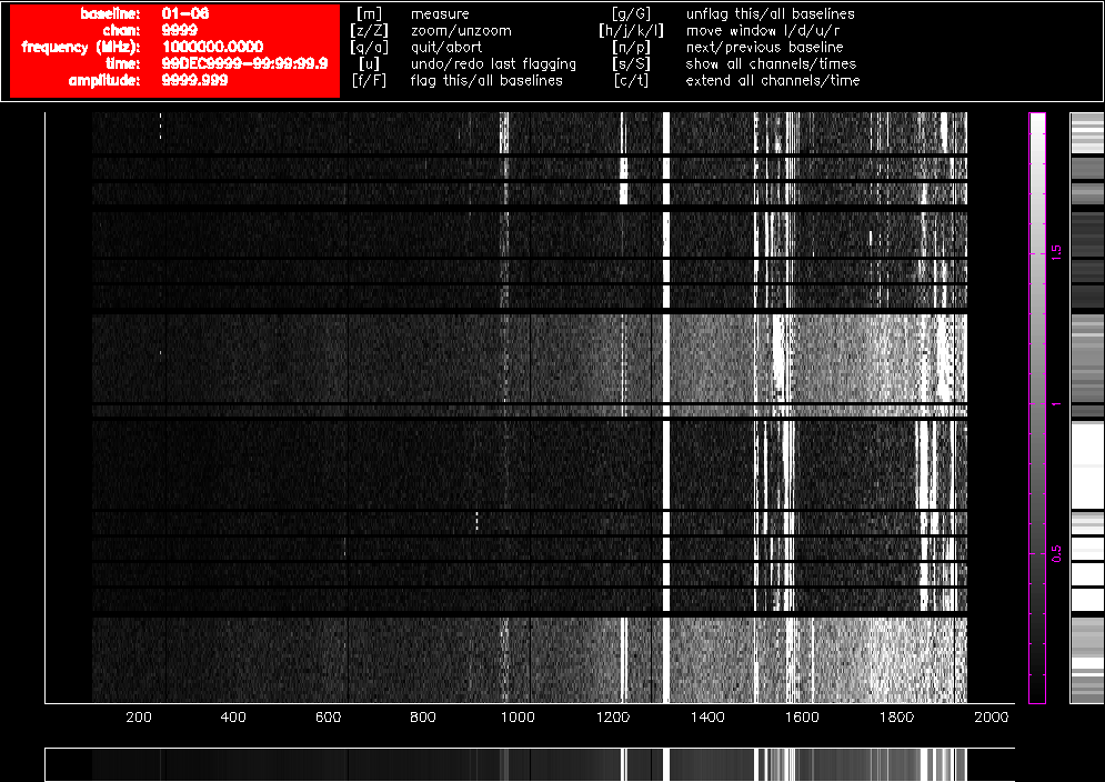
Figure 4.2. A pgflag display showing Stokes V data on a long baseline in a 16cm dataset before flagging.

After using pgflag as described above on the uncalibrated data, then bandpass calibrating and flagging with pgflag in the same way again, the data on the same baselines look like Figure 4.3 and Figure 4.4. Approximately 40% of the short baseline data is now flagged, and approximately 25% of the long baseline data.

Figure 4.3. A pgflag display showing Stokes V data on a short baseline in a 16cm dataset after flagging and bandpass calibration.

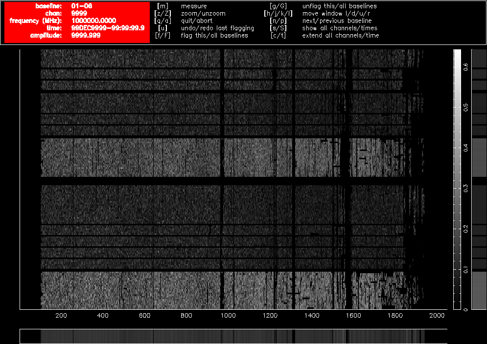
Figure 4.4. A pgflag display showing Stokes V data on a long baseline in a 16cm dataset after flagging and bandpass calibration.

As you can see, no obviously wrong signals can be identified in Stokes V after this process, but that does not necessarily mean that all RFI has been deleted from the data. Figure 4.5 and Figure 4.6 show Stokes Q on the same baselines as before, after the Stokes V flagging and bandpass calibration, and further RFI is obvious in those figures. We now flag using the linear-polarisation Stokes parameters Q and U.

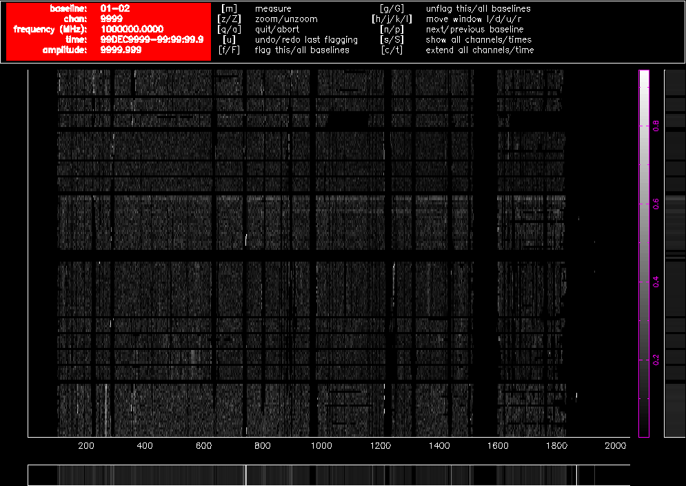
Figure 4.5. A pgflag display showing Stokes Q data on a short baseline in a 16cm dataset after flagging in Stokes V and bandpass calibration.

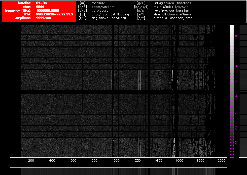
Figure 4.6. A pgflag display showing Stokes Q data on a long baseline in a 16cm dataset after flagging in Stokes V and bandpass calibration.

To do this we use pgflag as follows. First, flag Stokes Q:

$ pgflag stokes=i,v,u,q flagpar=8,2,2,3,6,3 "command=<b"

And then Stokes U:

$ pgflag stokes=i,v,q,u flagpar=8,2,2,3,6,3 "command=<b"

Again, these flagging commands can be done on each source individually, or on the dataset as a whole.

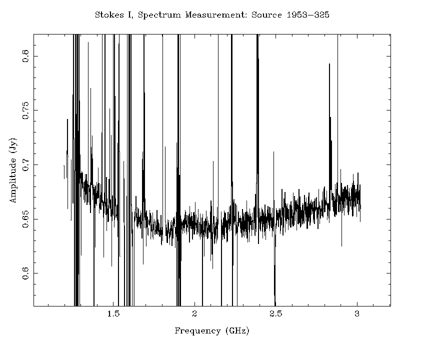
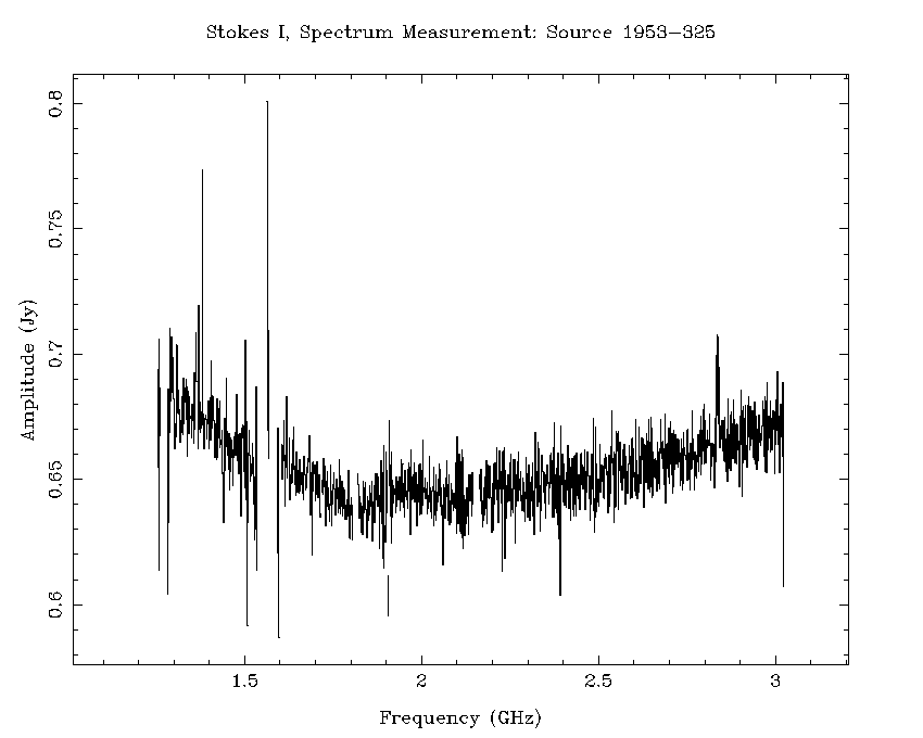
An example of how effective this flagging recipe can be is shown in Figure 4.7 and Figure 4.8. Using the calibration solutions derived from the flagged dataset, we can compare the 16cm spectrum of the calibrator 1953-325 before any flagging (Figure 4.7) to the spectrum after flagging (Figure 4.8). After the flagging process, only a small amount of RFI remains, and this is not likely to cause problems when measuring the continuum spectrum. On the shortest baselines, between 45-50% of the data has been flagged, but on the baselines to antenna 6 less than 30% of the data needed to be flagged. In terms of channels, 1625 of the channels have usable data out of the 2049 total channels, representing a spectral coverage loss of approximately 21%.

Figure 4.7. The 16cm spectrum of the source 1953-325 without any flagging.

Figure 4.8. The 16cm spectrum of the source 1953-325 after automatic flagging with pgflag.

The calibration strategy for ATCA data has been refined for the CABB era, to ensure accurate calibration of wide bandwidths. This strategy also has the benefit of being applicable to the vast majority of ATCA data with little alteration. It is described best in the Miriad cookbook, but it will also be summarised here (although not explained in the same depth).

Task:   mfcal
vis      = 1934-638.2100/
line     =  
stokes   =  
edge     =  
select   =  
flux     =  
refant   =  
minants  =  
interval = 0.1
options  =  
tol      =  

Task:   mfcal
vis      = 1921-293.17000/
line     =  
stokes   =  
edge     =  
select   =  
flux     =  
refant   =  
minants  =  
interval = 0.1
options  =  
tol      =  

Task:   gpcal
vis      = 1934-638.2100/
select   =  
line     =  
flux     =  
refant   =
minants  =  
interval = 0.1
nfbin    = 2  
tol      =  
xyphase  =  
options  = xyvary

Task:   gpcopy
vis      = 1921-293.17000
out      = 2243-123.17000
mode     =  
options  =  

Task:   gpcal
vis      = 2243-123.17000/
select   =  
line     =  
flux     =  
refant   =
minants  =  
interval = 0.1
nfbin    = 2  
tol      =  
xyphase  =  
options  = xyvary,qusolve

4.3.2.6.3. Flux density calibration

4.3.2.6.3.1. Calibration in the cm bands

If you used 1934-638 in the mfcal and gpcal steps, then you already have a flux calibrated dataset that can be used to fix the flux density scale on the other datasets.

You should now copy the solutions from the 1934-638 dataset to the gain calibrator dataset using gpcopy, and determine the time-variable gains with gpcal.

Task:   gpcopy
vis      = 1934-638.2100/
out      = 2243-123.2100/
mode     =  
options  =

Task:   gpcal
vis      = 2243-123.2100/
select   =  
line     =  
flux     =  
refant   =
minants  =  
interval = 0.1
nfbin    = 2  
tol      =  
xyphase  =  
options  = xyvary,qusolve

The gpcal step is likely to make the flux density scale on your gain calibrator slightly different to the true scale. To fix this you should use gpboot.

Task:   gpboot
vis      = 2243-123.2100/
cal      = 1934-638.2100/
select   =  

You can now be confident that your gain calibrator is properly flux calibrated, and can now proceed to use it to analyse your science target.

4.3.2.6.3.2. Calibration in the mm bands

At this point in the mm reduction, you need to do the flux density calibration. How this happens depends on whether you're using a planet as the flux density calibrator, or 1934-638. After copying the calibration tables from the calibrator used in the gpcal step to the flux density calibrator, you use gpcal followed by gpboot if you're using 1934-638, or mfboot for planets.

1934-638 flux calibrator	planetary calibrator
Task: gpcopy vis = 2243-123.17000/ out = 1934-638.17000/ mode = options = Task: gpcal vis = 1934-638.17000/ select = line = flux = refant = minants = interval = 0.1 nfbin = 2 tol = xyphase = options = xyvary,qusolve,nopol Task: gpboot vis = 2243-123.17000/ cal = 1934-638.17000/ select =	Task: gpcopy vis = 2243-123.33000/ out = uranus.33000/ mode = options = Task: mfboot vis = 2243-123.33000,uranus.33000/ line = select = source(uranus) flux = mode = clip = device = /xs options =

Note the use of the nopol option for the options parameter in gpcal, when 1934-638 is being used as the flux density calibrator. This option tells gpcal that it should accept the leakage solution obtained from the gain calibrator, which should be good since the gain calibrator is likely to have much greater hour-angle coverage than the flux density calibrator.

In May 2016, Miriad's high-frequency flux density scale for 1934-638 was changed to align the ATCA's scale to that of the VLA and the absolute scale used by Planck. See Section 2.2.4 for details about this new scale. By default, after May 2016, Miriad uses this new scale when setting the flux density of 1934-638 for frequencies above 11 GHz. The flux densities measured from reductions using pre-May 2016 and post-May 2016 Miriad will therefore differ for observations above 11 GHz. If you would like to keep using the pre-May 2016 flux density scale for 1934-638, you should use the oldflux option that is available in the mfcal, and gpcal commands.

At this point the gain calibrator will be reasonably well calibrated. If you are not especially concerned about flux density calibration accuracy, you can proceed to analyse your science target.

If you want to flux calibrate your data as well as possible, then you can use data from the other simultaneously observed band to improve your solution. Basically, the bandpass solution you made earlier assumed that the bandpass calibrator had a constant flux density with frequency (i.e. a flat-spectrum source). Because of this, the bandpass solution will likely be in error. Our gain solutions with two bins will have corrected this somewhat, but we can also try to emulate the situation in the cm band, and provide mfcal with a model of the flux density of the bandpass calibrator.

To do this, we copy the gain solutions from the gain calibrator back to the bandpass calibrator, recalibrate, and bootstrap the flux density scale.

Task:   gpcopy
vis      = 2243-123.17000/
out      = 1921-293.17000/
mode     =  
options  =

Task:   gpcal
vis      = 1921-293.17000/
select   =  
line     =  
flux     =  
refant   =
minants  =  
interval = 0.1
nfbin    = 2  
tol      =  
xyphase  =  
options  = xyvary,qusolve,nopol

Task:   gpboot
vis      = 1921-293.17000/
cal      = 2243-123.17000/
select   =  

Note that these steps don't change regardless of the type of flux density calibrator you are using.

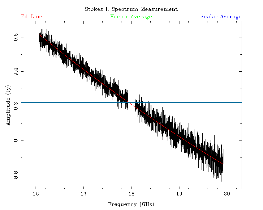
You should do the same calibration process with the other simultaneously observed band. At the end of the process you should have two bandpass calibrator datasets, each being flux density calibrated via the gain calibrator. You can now measure the flux density of the bandpass calibrator over the entire range of observed frequencies, using the uvfmeas task. The principle here is that even if the slope over a single band is wrong due to the incorrect bandpass calibration assumption, fitting a flux density model using two independently-calibrated bands should lower the uncertainties and provide a very good model of the actual flux density of the source.

Task:   uvfmeas
vis      = 1921-293.17000/,1921-293.19000/
select   =  
line     =  
stokes   = i
hann     =  
offset   =  
order    = 1
options  = plotvec,log,mfflux
yrange   =  
device   = /xs
nxy      =  
log      =  
fitp     =  
feval    =  

The uvfmeas task does a linear least-squares fit to the log of the vector-averaged Stokes I flux density as a function of the log of the frequency. The plot it makes will show the averaged data in both bands, and the line of best fit (Figure 4.9). It will also output a string like:

MFCAL flux= 9.4126, 17.0,-0.3801

Figure 4.9.  A plot made using uvfmeas, showing the line of best fit for the flux density model.

The string is usable as the flux in mfcal, which will fit the bandpass solution while assuming the flux density model we just determined. The image in Figure 4.9 is actually the result of this two stage process, and you can see the excellent alignment between the two bands, which are independently processed.

Once you have measured the flux density model for the bandpass calibrator, you must redo the calibration, but the bandpass calibrator becomes the flux density calibrator. The process is slightly different as well, and is summarised below.

Task:   mfcal
vis      = 1921-293.17000/
line     =  
stokes   =  
edge     =  
select   =  
flux     = 9.4126,17.0,-0.3801
refant   =  
minants  =  
interval = 0.1
options  =  
tol      =  

Task:   gpcopy
vis      = 1921-293.17000/
out      = 2243-123.17000/
mode     =  
options  =

Task:   gpcal
vis      = 2243-123.17000/
select   =  
line     =  
flux     =  
refant   =
minants  =  
interval = 0.1
nfbin    = 2  
tol      =  
xyphase  =  
options  = xyvary,qusolve

Task:   gpcopy
vis      = 2243-123.17000/
out      = 1921-293.17000/
mode     =  
options  =

Task:   gpcal
vis      = 1921-293.17000/
select   =  
line     =  
flux     =  
refant   =
minants  =  
interval = 0.1
nfbin    = 2  
tol      =  
xyphase  =  
options  = xyvary,qusolve,nopol

Task:   gpboot
vis      = 2243-123.17000/
cal      = 1921-293.17000/
select   =  

Task:   mfboot
vis      = 2243-123.17000,1921-293.17000/
line     =  
select   = source(1921-293)
flux     = 9.4126,17.0,-0.3801
mode     =  
clip     =  
device   = /xs
options  =  

At this point both the bandpass and gain calibrator datasets will be very accurately flux density calibrated. Simulations suggest that this two-stage process can improve the flux density calibration accuracy to the 1% level for the bandpass calibrator, and to around the 3% level for any other calibrators referenced to it. Observations have confirmed this in the 15mm band, while for the 7mm band the flux calibration accuracy for an arbitrary gain calibrator is around 10%.

Imaging of CABB data can be performed in exactly the same way as pre-CABB data, however you may get better results with a slightly different method.

For high-frequency observations, where a bandwidth of 2 GHz does not represent a very large fraction of the sky frequency, then the imaging strategy used for pre-CABB data will most likely be adequate. For lower frequencies the multi-frequency strategies are more likely to produce good results. In particular, the use of the mfclean task should be considered. Read the excellent description of why mfclean is necessary in the Miriad cookbook to see if you will need to proceed with this strategy.

If you don't need mfclean then you should proceed with the usual invert, clean and restor method of creating an image, and combine this with selfcal or gpscal if appropriate. In this case, nothing should be different from pre-CABB reduction.

If you do need mfclean then the inputs to invert will need to be slightly different as well. Firstly, both the mfs and sdb options will need to be passed to invert. mfclean also requires that the beam be three times the size of the region being cleaned, which can be quickly specified in the latest version of Miriad in the imsize.

Task:   invert
vis      = obs.uv
map      = obs.map
beam     = obs.beam
imsize   = 3,3,beam
cell     = 
offset   =
fwhm     = 
sup      = 
robust   = 0.5
line     =
ref      =
select   = 
stokes   = i
options  = mfs,sdb
mode     =
slop     =

The first two options to the imsize parameter are usually the number of pixels in the x and y direction respectively that the image will have. But when you specify the beam option as the third argument to imsize, the first two options are interpreted as multiples of the FWHM of the primary beam at the central frequency of the image. In the example above, both the dirty image and the synthesised beam image would cover 3 times the primary beam FWHM in each direction. In earlier versions of Miriad, both the imsize and cell parameters would have needed to be determined manually and explicitly set to do the same thing.

With the synthesised beam covering 3 times the primary beam FWHM, mfclean can be used to clean the entire primary beam.

Task:   mfclean
map      = obs.map
beam     = obs.beam
model    =
out      = obs.clean
gain     =
cutoff   =
niters   =
region   = percentage(33)
minpatch =
speed    =
mode     =
log      =

Here we are selecting the central third of the image (the primary beam area) with the region keyword. This also satisfies the mfclean requirement that a guard band be present around the region being cleaned. The other parameters are very similar to those of clean and should be set as usual to obtain good results.

After mfclean has run, restor should be used in the normal way to produce the cleaned image. selfcal can also be used in the usual fashion in this process.