At the start of observing, a number of procedures need to be executed to set up the array for observng. The following table summarises the tasks, and indicates the wavelengths which need the various tasks.
| 16cm | 6&3cm | 15&7mm | 3mm | ||
| Set focus | ✔ | ✔ | ✔ | ✔ | See Section 3.3.1 |
| Set CABB attenuator levels | ✗ | ✔ | ✔ | ✔ | See Section 3.3.2 |
| Set CABB channel ranges | ✔ | ✔ | ✔ | ✔ | See Section 3.3.3 |
Check delavg | ✔ | ✔ | ✔ | ✔ | See Section 3.3.4 |
| Flag interference | usually not necessary | See Section 3.3.5 | |||
| Calibrate delays | ✔ | ✔ | ✔ | ✔ | See Section 3.3.6.1 |
| Check pointing | ✗ | ✗ | ✔ | ✔ | See Section 3.3.6.2 |
| Calibrate phases | ✔ | ✔ | ✔ | ✔ | See Section 3.3.6.3 |
| Calibrate gains | ✔ | ✔ | ✔ | paddle | See Section 3.3.6.4 |
The subreflector on each of the ATCA antennas can be raised and lowered to allow the signal to be focussed at the receiver feed. However, changing the subreflector position will change the path length (obviously) which will change the geometric phases and delays, so, it should only be done when required, usually when the frequency changes. Extra care is needed with calibration with programs that change focus during the observation.
A good time to do this is at the start of the observing and it can be done while driving to source.
Default focus positions have been determined for each band.
caobs> focus default | drives the subreflector to the default focus height for that band | |
caobs> focus ca0# | drives the subreflector on antenna # to the given focus height in mm |
Table 3.1. Subreflector Focus Positions for the Antennas.
| Ant | 16cm | 4cm | 15mm | 7mm | 3mm |
|---|---|---|---|---|---|
| CA01 | 17.0 | 4.1 | 17.8 | 17.0 | 14.0 |
| CA02 | 10.0 | -1.9 | 10.7 | 9.8 | 10.0 |
| CA03 | 10.0 | -2.2 | 10.4 | 9.0 | 9.0 |
| CA04 | 23.0 | 10.6 | 23.0 | 23.0 | 23.0 |
| CA05 | 18.0 | 7.1 | 20.2 | 18.5 | 18.4 |
| CA06 | 22.5 | 7.0 | 20.5 | 22.5 | 22.5 |
Note: As the antenna tips over, it deforms slightly, and the detected focus position changes by up to 1mm. This is normal and will not significantly affect the data.
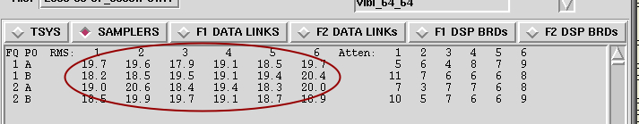
The rms digitiser quantisation levels (as displayed in the
sampler tab of cacor; see Figure 3.2) should be close to 20
(Range: Approximately 15-25).
To set the levels, attenuation can be added or removed.
The values in the Atten section of the window show the settings of the cacor
attenuators. They have a range of 0-15 dB.
For 16cm observations, strong RFI in the band will often make the sampler levels vary
significantly from cycle to cycle, making it difficult
(and often impossible) to set the attenuators appropriately.
It is therefore recommended to skip this step when observing at 16cm.
However, in rare cases the attenuator settings shown in the Atten section
could be quite low (all values far below 7), and at those times it could be useful to reset them either
automatically or manually as described below.
For all other bands, if the levels are not close to 20, the ATTS button in the cacor GUI can be activated to enable cacor to automatically add or remove attenuation.
This can also be done in the cacor interface:
cacor> tatts[ervo] 20 | set the target for the attenuator servos to 20 | |
| (most of the time, this command is not needed as tatts will usually already be set to this level) | ||
cacor> atts[ervo] on | correlator servos the attenuators to adjust the levels into the samplers |
Wait for the levels to settle to around 20, then turn the adjustment off again with:
cacor> atts[ervo] off |
Fairly obviously, the algorithm is unable to “improve” the levels if the attenuators are at their limits (0 or 15).
As noted above, strong RFI in the 16cm band makes it difficult to set the attenuators appropriately.
High values of attenuator settings, even up to the maximum value of 15, are not harmful.
However, you can also set the attenuators manually to values that
are known to be good, as listed in Table 3.2. To set the attenuators manually, you will need to
use the att command. For example, to set the CA03 attenuators as per Table 3.2,
you would need to give the commands:
cacor> att1 ca03 6 13 | sets the CA03 IF1 A and B pol attenuators | |
cacor> att2 ca03 2 2 | sets the CA03 IF2 A and B pol attenuators |
See
att
for more complete information about how to use this command.
f ca0# n m
Table 3.2. Attenuator settings for the 16cm band
| Product | CA01 | CA02 | CA03 | CA04 | CA05 | CA06 |
|---|---|---|---|---|---|---|
| 1 A | 5 | 4 | 6 | 7 | 8 | 6 |
| 1 B | 9 | 3 | 13 | 5 | 9 | 8 |
| 2 A | 10 | 4 | 2 | 9 | 8 | 4 |
| 2 B | 7 | 4 | 2 | 5 | 9 | 4 |
If the sampler levels are very low (approx 0), there is probably a problem which will need to be checked.
There are another set of attenuators in the receivers (as opposed to the correlator) which can also be used to set the levels.
These are controlled from caobs.
caobs> show atten[uation] | shows the current receiver attenuation levels in the caobs status window |
caobs> set atten ca0# atta attb | sets the receiver attenuator levels on antenna # to attenuator levels a and b. This value will be the same for both IFs. |
cacor generates an average visibility (either the mean or the median across the spectrum) that is used for Tsys and array calibration. In general, the median is much more stable and allows for a more reliable calibration. Otherwise, care needs to be taken to ensure that the range of cacor channels used for calculating the average is as wide as possible within the useable passband, but also excludes interference.
The default behaviour is to compute the average across the spectrum. To ensure that the more stable and reliable
median is being used, it is recommended to enable the tvmedian option:
cacor> tvmedian on on | Two arguments are required to enable the median option for both frequencies. |
At higher frequencies and when the tvmedian option is enabled,
it is usually appropriate to use the central fifty percent of channels.
The easiest way to do this is to type
cacor> tvch[an] default | sets the channel range to use the central 50% of the channels (i.e. channels 513 - 1537). |
Alternatively if tvmedian is disabled (not recommended), the information below can be
referred to.
At cm frequencies, interference means that it is often better to select
non-default channels, when tvmedian is disabled (not recommended).
See Table 3.3 for information on recommended channel ranges for 2048 MHz continuum bands.
If these channel ranges are not generating the anticipated visibility in vis, inspect Appendix C to
determine the cause of the problem.
The tvchan command sets the range of channels that are used for
calibrating the array and for Tsys calculation. The same range is used to
compute the average (or median) visibility for display in vis. All unflagged
channels are written to the data (RPFITS) file regardless of what the tvchan
setting is.
(Note: Channels that are flagged are written to the file as zeroes. See Section 3.3.5 for more information).
Current settings are displayed in the cacor GUI, as shown in Figure 3.3.
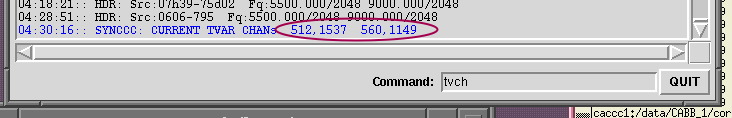
It is also possible to check the current setting with the cacor command
cacor> tvch[an] | The first pair of numbers gives the channel range for the first frequency. The second pair of numbers gives the channel range for the second frequency. |
Setting the range is done with the cacor command:
cacor> tvch[an] default | sets the channel range to use the central 50% of the channels (i.e. channels 513 - 1537). | |
cacor> tvch[an] ch1
ch2
ch3
ch4 | sets specific channels where ch1 and ch2 are the low and high channels for frequency 1 and ch3 and ch4 are the low and high channels for frequency 2. | |
cacor> tvch[an] f# ch1 ch2 | sets specific channels for a single frequency, where # is the frequency (1 or 2). |
Table 3.3 lists the suggested tvchan ranges for the standard continuum bands. On any given day (or interference environment) other ranges may be more appropriate.
Table 3.3. Suggested tvchan ranges for standard ATCA Continuum bands.
| Band | Centre Freq | 1 MHz channels | 64 MHz channels | ||
|---|---|---|---|---|---|
| (MHz) | ch1 | ch2 | ch1 | ch2 | |
| 16cm | 2100 | 200 | 949 | 2 | 14 |
| 6cm | 5500 | 513 | 1537 | 9 | 25 |
| 3cm | 9000 | 200 | 1149 | 9 | 25 |
| 15mm | 17000 | 513 | 1537 | 9 | 25 |
| 7mm | 33000 | 513 | 1537 | 9 | 25 |
| 3mm | 93000 | 513 | 1537 | 9 | 25 |
(There is a wide range of valid frequency settings at mm frequencies).
To calculate the delay of an individual IF, cacor
checks the phase in each channel in the tvchan range
(just defined) and calculates an average linear slope from
the phase measurements as a function of frequency; this slope is the delay.
If the noise on the phase is high (due to a faint source or poor weather, for example)
or there is some strong unavoidable RFI in the tvchan
range, then the average slope may not accurately represent the real
slope due to the delay.
To reduce the noise, or to average out the effect of the RFI, setting delavg in the correlator
averages together (or takes the median of) the corresponding number of channels in the
tvchan range before calculating the slope to determine the delay.
Here too it is useful to use the median option rather than the default mean (computed within each
group of delavg channels):
cacor> tvmedian on on | Two arguments are needed to enable the median option for both frequencies. |
Higher values of delavg can be useful for determining the delays.
However, care needs to be taken when selecting this value!
If the phases are wrapping quickly, averaging over a
large number of channels will give a meaningless average phase, and therefore incorrect
delays will be determined.
The current value of delavg is in the status bar of the cacor interface.
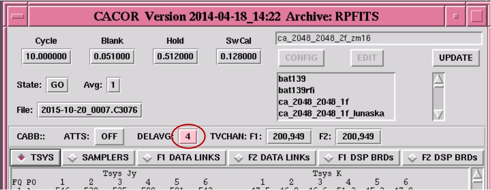
Setting delavg is done with the cacor command:
cacor> delavg # | Averages # channels. |
|
|
| |
|
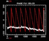
An spd plot demonstrating slow changes in phase.
The phases are not wrapping at all in the A pol, and wrapping approximately every 250 channels in the B pol.
Averaging over 32 channels would still provide enough points across the band to achieve a useful linear fit to the data, so |
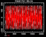
An spd plot demonstrating rapidly wrapping phases. The phases in both pols of this graph are wrapping across a small number of channels. It is possible to check just how quickly the phases are wrapping by viewing a smaller number of channels:
spd
The value of |
Occasionally, there will be channels that, because of interference (or other issues), you may wish to completely excise from the data (i.e. not write those channels to the data file).
To check the extent of currently flagged channels:
cacor> fflag | display the number of channels that are currently unflagged. In each frequency, there is a maximum of 2049 channels. |
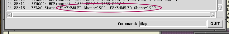
There is no easy way to discover which channels have been flagged, and flagging will remain even with a change of project (or frequency etc.) so flagging should be checked at the start of observing. If there are more channels flagged than anticipated, flagging should be cleared then reflagged if necessary.
This is done by:
cacor> fflag f# default | flags the central channel (and 1/4, 3/4 channels) in frequency # |
To flag the set of known bad continuum channels
cacor> fflag f# birdies | flags channel known bad channels in frequency # |
This needs to be done at both f1 and f2.
To flag explicit channels, use the command:
cacor> fflag f# chm | flags channel chm in frequency # | |
cacor> fflag f# chm-chn | flags channels chm to chn
inclusive in frequency # |
Again, this needs to be done at both frequencies.
If you know exactly which channels have been flagged, they can be unflagged with the
funflag command: formats are similar to the fflag command i.e.
cacor> funflag f# chm | unflags channel chm in frequency # |
Once the array is working, the system can be calibrated.
Calibration will not fix a broken system.
The calibration involves calculating and applying the delay offsets, checking the pointing (for mm observations), setting the phases to zero degrees and correcting the visibility amplitudes to the appropriate flux levels.
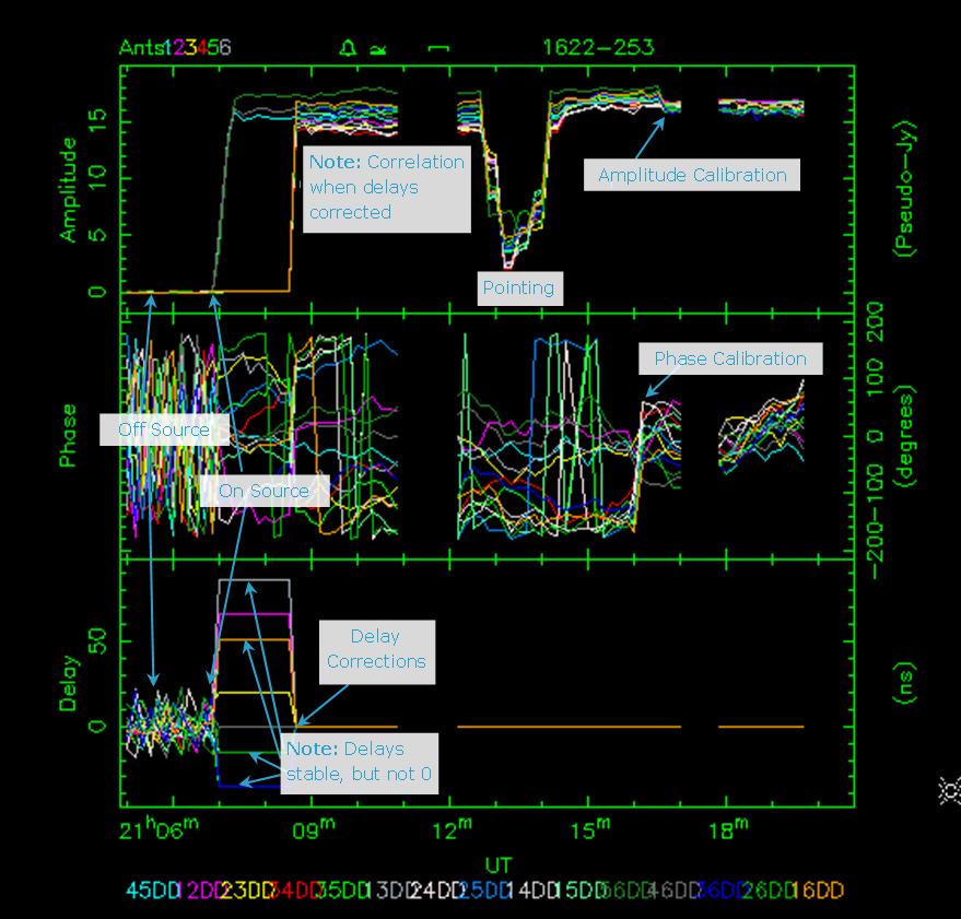
Delay offsets need to be determined and corrected at the start of the observation. Failure to correct for delay offsets may result in decorrelation, and loss of data.
In the 64MHz zoom configuration, delay calibration is more complex as it generally needs to be done in two steps. (First delay calibrate a zoom channel, then in the continuum. See Section 3.3.6.1.1 for more information)
To calibrate the delays, track an unresolved source with large flux density
(e.g. PKS1934-638 or PKS0823-500 for cm
observations; for mm observations use PKS1253-055,
PKS1921-293, PKS2223-052 or
PKS0537-441).
PKS1934-638 and PKS0823-500
do not have enough flux density to calibrate at mm frequencies.
Correlation should be apparent before you proceed. Phases in spd should be stable, though they may be wrapping rapidly and delays should be flat in vis. Check that you have correlation in both frequencies and both polarisations.
If there is significant interference (see the amplitude plot in spd), you will need to carefully craft the tvchan range (or, if bad enough, actually flag interfering channels) to avoid the interference in the calibration data.
If working at 3mm or with significant interference, it may be necessary to average over several channels (to improve the signal/noise ratio) with the command:
caobs > corr delavg # | where 8 is a good initial value for # - however,
if the delays are large (>50nsec), you should try a smaller value to start with. |
If you still don't have correlation, check Section 3.5.6 at the end of this chapter, and if this doesn't resolve your problems get help.
Assuming that the phases in spd are stable, enter the command:
caobs > corr dcal | dcal calculates and applies the required correction. |
This command should correct the delays so that the phases across the band on the spd plot are flat (or fairly close to flat) and the delay offsets as seen on vis are close to 0 nsec. It may be necessary to do this again.
(Early versions of the CABB software required an “a” switch at the
end of the dcal command for the correction to actually be applied.
The delays are now applied automatically by the command. Any switch other than an
a will result in the delays not being applied.)
Delay calibration is slightly more complex in 64MHz mode.
The issue is that typical delays can cause the phases to wrap more than once within a single
(64MHz wide) continuum channel. As is the case when delavg is set too high in 1MHz mode,
a valid delay solution cannot be determined in this circumstance.
The solution for this is to obtain an initial solution for the delays using zooms, which will unwrap
the phases sufficiently to be able to determine the delays using the continuum channels.
The process is illustrated in Figure 3.9 to Figure 3.13.
To use the zooms for delay calibration, set calband to z z:
cacor > calband z z | Uses zoom data in both frequencies. For a hybrid correlator config, use f z |
Do the delay calibration as normal.
At this stage a large value of delavg is often acceptable.
caobs > corr dcal | As always, ensure that there is a working system before doing the dcal |
|
|
| |
|
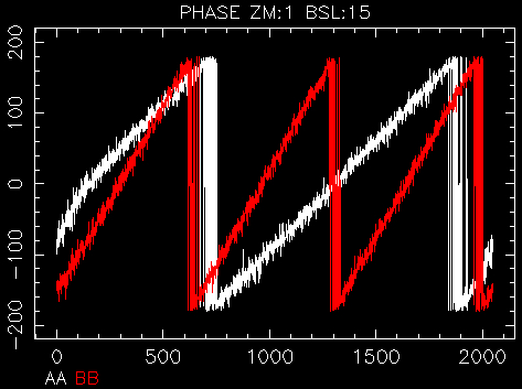
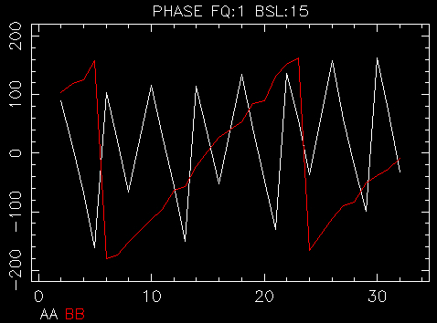
An spd plot demonstrating typical phase variations across a zoom band. In this case the delays are large enough that the phases wrap multiple times across the zoom band, and thus are also wrapping multiple times within the corresponding 64MHz-wide continuum channel. |
An spd plot showing the zoom band phases after delay calibration. After performing delay calibration on this zoom band, the phases have been flattened across the 64MHz range. |
Once the majority of the delay error has been corrected for, the whole continuum band needs to be used for a second delay calibration:
cacor > calband f f | ||
caobs > corr dcal |
Pay attention to the value of delavg at this step to ensure that it is sufficiently low.
There are only a handful of channels to work with in the continuum bands in this mode!
|
|
|
| ||
|
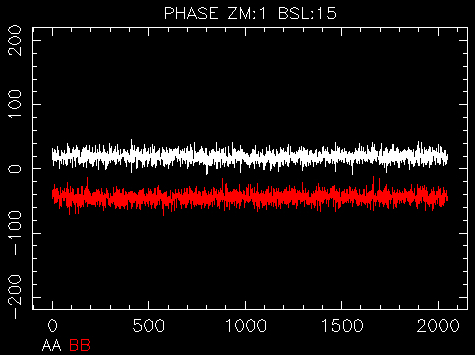
Continuum band phase variations before delay calibration. This is the continuum band corresponding to the zoom band shown in Figure 3.9. It is clear (especially for the A polarization) that before any delay calibration, the average phases within each 64MHz continuum channel are not useful to determine a delay solution. |
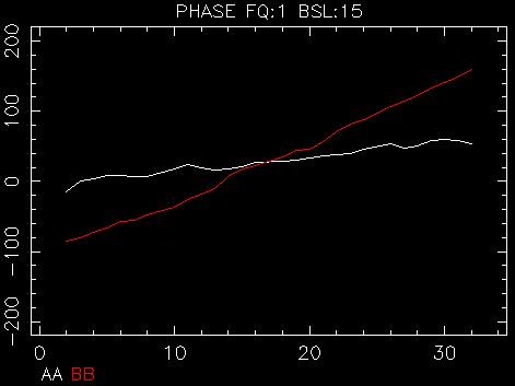
Continuum band phase variations after zoom-band delay calibration. After performing delay calibration on the zoom bands, the phases have been largely flattened. The delays determined across a 64MHz frequency range are not sufficient to fully calibrate the continuum band, but they are sufficient to allow a refined delay calibration over the full continuum frequency range. |
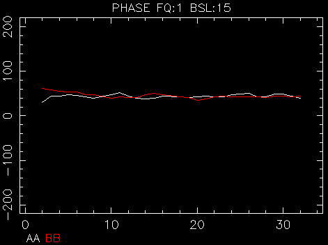
Continuum band phase variations after final delay calibration. After performing a further delay calibration on the continuum bands, an excellent solution has now been obtained. This is apparent from the flatness of the phases across the full frequency range. |
If observing at mm wavelengths, the antenna pointing should be checked and corrected before phase and amplitude calibration. A pointing scan has six separate pointings: first on the nominal on-source position, followed by four pointings at the nominal half-power points (+/- Az, +/- El), then a pointing back on the on-source position. A separate task, catag, calculates the pointing offets and feeds them back to the system to be implemented.
Check the pointing [1] page in MoniCA to check that the appropriate catag parameters are set:
User Antenna Maskshould include all antennas that need to be used for pointing.User IF Maskshould be set to include IFs that are required. 1234 uses all 4 IFs. 12 uses the two polarisations in the first frequency. 34 uses both polarisations in the second frequency. The setting 1234 can only be used if the frequenciesf1andf2satisfy .Integration Cyclesdefines the number of cycles spent on each step of the pointing solution. This will usually be set to 2 or 3.
Modifying these parameters is done in caobs
caobs > set point_a a1[a2
...a6] | defines antennas to be included in pointing calculations | |
caobs > set point_a 12345 | would use all antennas except CA06 |
Note: Pointing using the selfcal algorithm (default mode) requires 4
or more antennas to calculate gains. If using 3 or fewer antennas, holography mode is needed.
To enable holography, set the Integration Cycles to the negative (e.g. -2) value.
caobs > set point_if if1[if2...
if4] | defines IFs to be included in pointing calculations; | |
caobs > set point_if 1234 | would use both frequencies, both polarisations. |
(Note: If the two frequencies are different by more than 15%, the system will not let you use the second frequency. This is because the beam size is sufficiently different that problems can arise - think about the situation of a 5 and 10 GHz frequency pair. The half-power point at 5 GHz is the first null at 10 GHz.)
caobs > set point_p # | where # is the number of cycles spent on each pointing step. # is usually 2 or 3. If using holography mode, this should be -2 or -3. |
After these parameters have been set, ensure that your schedule file has a pointing scan set up.
This scan will need to have “Scan Type” set to “Point” and
the “Pointing” parameter set to “Update”.
To start the pointing scan, you must use the “start” command in caobs
(“track” will simply track the on-source position):
caobs > start # | where # is the scan number of the pointing scan. |
Watch the amplitudes in vis to check progress. You should see the amplitudes drop to approximately half the amplitude of the nominal centre position. The difference between the plus and minus pointings give an indication of the error in the pointing.
After the pointing scan has finished, check the errors that are found in the MoniCA pointing page. If any of the “Last Az Correction” or “Last El Corrections” is greater than 10″, a second pointing should probably be considered.
For more information on offset pointing, see the Reference Pointing Guide.
Phase Calibration is somewhat “cosmetic”, however, it can be useful to set the phases to zero at the start of observations to help judge the phase stability. To set the phases to zero:
caobs > corr pcal | pcal calculates the required correction and
applies the correction that the pcal offsets. |
(Early versions of the CABB software required an “a” switch at the
end of the acal command for the gains to actually be applied.
They are now applied automatically by the pcal command. Any switch other than an
a will result in the phase corrections not being applied.)
Once the delays have been set and pointing checked (for mm observations), the antenna gains need to be set. To set the gains:
caobs > corr acal [#1 #2] | acal calculates the required correction.
#1 and #2 are the fluxes of the calibrator
at the first and second frequencies respectively. |
(Early versions of the CABB software required an “a” switch at the
end of the acal command for the gains to actually be applied.
They are now applied automatically by the acal command. Any switch other than an
a will result in the gain corrections not being applied.)
If using PKS1934-638 or PKS0823-500,
the flux densities are known by caobs and do not have to be entered, i.e.
caobs > corr acal |
Gain settings are used for calculating Tsys. This can be recalculated off-line, but some care needs to be taken.
The Tsys values should be checked in the cacor GUI.
Any outlier readings should be checked.
At this point, the array should be set up and ready for observing. Check that all the products in vis look correct and that the Tsys values (in cacor) are appropriate. If there are any problems, check the Troubleshooting section Section 3.5.6 or get help.
When you have concluded setting up for observations and are prepared to begin observing, it is good practice to close the data file produced by the correlator so that the data produced during the setup process is not confused with useful calibrator and target data.
caobs> stop | ||
caobs> corr closefile | Closes the data file being written by the correlator in preparation for science observations. |