The Compact Array Broadband Backend (CABB)
What is CABB?
The Compact Array Broadband Backend (CABB) upgrade has provided a new broadband backend system for the ATCA. The maximum bandwidth of the ATCA was increased from the 128-MHz (in each of two IF bands) to 2-GHz, a factor of 16 improvement. This, coupled with higher level data sampling, has improved the continuum sensitivity of the ATCA by at least a factor of four as well as providing a greatly enhanced spectral line performance, particularly at the higher observing frequencies. The wider bandwidth allows projects studying spectral lines within a 2-GHz band to be carried out simultaneously.
The MOPS spectrometer in use at Mopra is largely a by-product of the development undertaken for the CABB upgrade project.
Quick Links
- CABB Current Status
- Important note about scheduling CABB observations
- What is available currently semester?
- Notes on calibrating 64 MHz mode
- Overview of CABB specifications
- The ATCA Users Guide provides information on CABB observing
- The ATCA forum (note -- moved in late May 2011 to a new URL) contains discussions on a number of issues related to CABB observing and data reduction
- The Miriad manual has been updated for CABB data reduction. (See the email sent to observers on May 31st regarding a bug that in mfcal between 13 April and 23 May 2011)
- A paper giving a detailed description of the CABB system and early science results with CABB has been published MNRAS vol. 416, p. 832 (2011). The preprint is available from the arXiv server. (The preprint refers in a couple of places to a CABB mode with "four IF bands (single polarization)" which does not exist -- this is corrected in the published version!) If you have a subscription to MNRAS you can access the published version.
- Schedule your observations with the CABB Scheduler. (You no longer need to be on the CSIRO network or have an ATNF unix account to access the tool.) Also see information about the CABB scheduler
- And always check the Current Issues page for the latest information
Important note about scheduling CABB observations
Note that although the CABB scheduler allows the CABB bandwidths to be specified, this information is currently not passed on to CABB -- reprogramming CABB between modes is at present a manual (and, in some cases, time consuming) process. The "Assistance" program will now warn if it finds an incompatability between the schedule file and the actual CABB mode. The ATCA schedule for a semester is assembled by scheduling projects using the same CABB mode in blocks and by leaving appropriate gaps for changes between modes: changes to the 1MHz zoom mode and 64 MHz zoom mode both require approximately one hour and these mode changes are done by local staff or suitably trained others. In the graphical version of the schedule the requested CABB mode is shown in the top right corner of each block. The mode "1M*" designates those proposals which requested a different mode (usually the 64MHz mode) but without justification, and so they have been allocated the 1MHz (no zooms) mode which is better suited to continuum observations. Observers who wish to change the CABB mode from that specified in the cover sheets of their proposal should contact the scheduler or ATCA local staff well in advance to see whether this will be possible.
What is currently available?
The CABB modes currently available are:
- CFB 1M (no zooms): A bandwidth of 2 GHz with 2048 x 1-MHz channels and in each IF band.
- CFB 1M-0.5k: A bandwidth of 2 GHz with 2048 x 1-MHz channels and (optionally) a fine resolution of 0.5 kHz (2048 channels across 1 MHz) in up to 16 "zoom" bands in each IF band.
- CFB 64M-32k: A bandwidth of 2 GHz with 32 x 64-MHz channels and (optionally) a fine resolution of 32 kHz (2048 channels across 64 MHz) in in up to 16 "zoom" bands in each IF band.
- CFB 1M/64M: A "hybrid" mode with 2048 x 1-MHz (but no zooms) in one IF, and 32 x 64-MHz channels with (optionally) up to 16 zoom bands with 2048 channels across each in the other IF.
- Pulsar binning: As for CFB 1M (no zooms) but with the addition of pulsar binning according to the provided ephemeris.
Notes on calibrating 64 MHz mode
The main difference with calibrating delays in 64 MHz mode (compared to the 1MHz modes) is that the "continuum" 64MHz bands are too coarse to determine anything but the smallest of delays. You may be lucky, if your observing freqs have been used recently, and the delays may be very small, but you should not assume this will be the case! For the source you are planning to use for delay calibration, add a single zoom channel (in the CABB scheduler) in each IF. (Channel 10, for example, with a width of 1.) After setting attenuators etc, in the cabb gui type calband z, z this will show (in vis) the zoom channels (each with 2048 channels across them). By default, the tvchan range will be something like 513 to 1535 for these zoom channels (but can be changed if necessary). In SPD, you can type sel z1 and sel z2 to show the phase and amp of each baseline. Make sure delavg is appropriately set, then dcal (in the CABb gui, or or corr dcal in caobs) will determine delays for those zoom bands and apply them (and show them in vis). Once you're happy with those, in the CABB gui type calband f, f in order to check the 32 x 64MHz channels in each IF. By default, the tvchan range is something like 9 to 24 for the 32 "continuum" channels (but can be changed if necessary). In SPD, sel f1 and sel f2 selects these. You will need to another dcal now to determine the delay solution across 2GHz rather then 64MHz. Once that's all done, the delays are calibrated and you can proceed.
Current Status
Sixteen zooms per IF in 64MHz mode
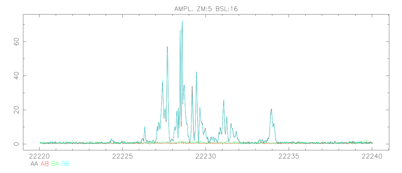
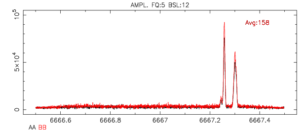
This plot shows a
sample of a CFB 64M-32k configuration,
with 16 zooms bands in each 2GHz IF band.
The plot shows a galactic centre water maser, with a 20MHz section of
a 64MHz zoom window shown, with a spectral resolution of 31.25 kHz
from observations on 13-sep-2012.
The blue and black spectra are the linear polarisations, and the red and green
spectra are the cross-polars
(courtesy Warwick Wilson & Dick Ferris).
Observers using the multi-zoom 64 MHz mode should tune their bands so
that selected zooms don't fall across the sampler birdies at 25%, 50%
and 75% of the 2048MHz span.
Sixteen zooms per IF in 1MHz mode
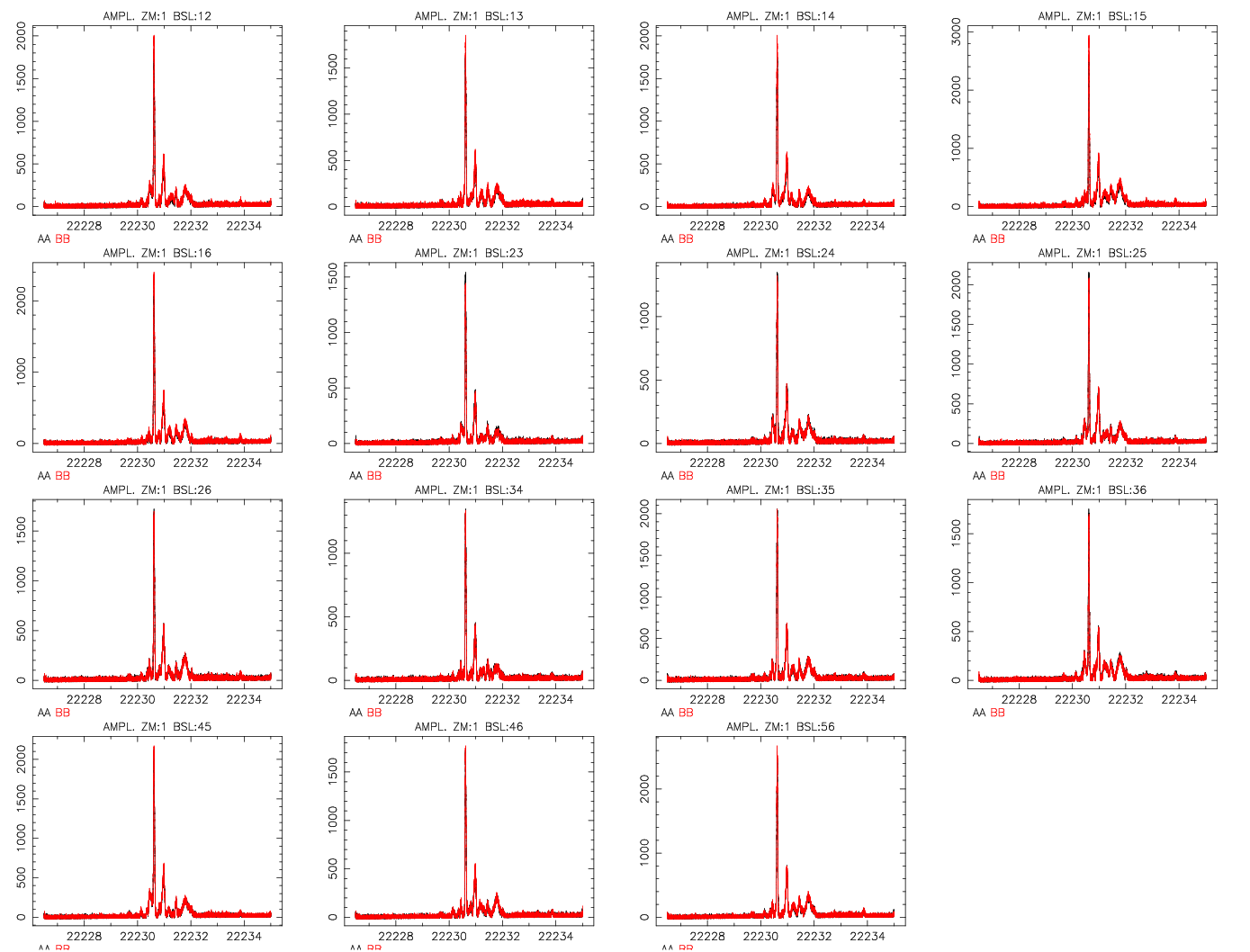
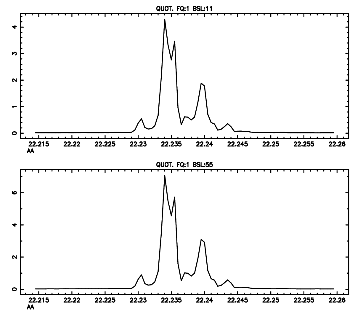
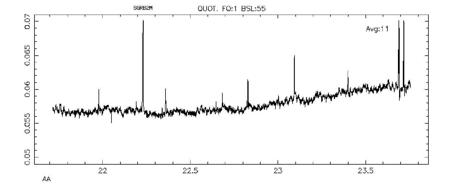
These plots show
the first 16*1 MHz zoom spectrum from CABB, of
water masers in Sag B2.
Sixteen 1 MHz zooms have been concatenated (i.e., overlapped in 0.5 MHz steps)
to give 17,408 channels over 8.5 MHz.
(courtesy Warwick Wilson & Dick Ferris).
Pulsar binning with CABB
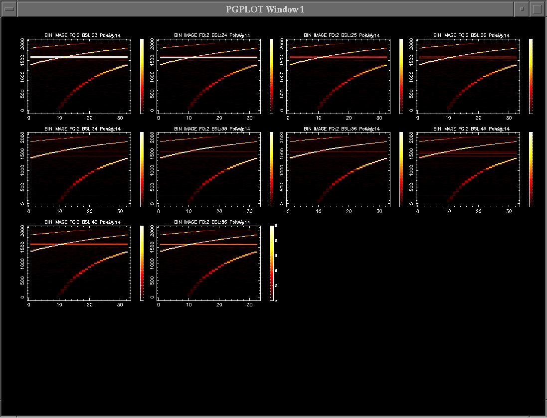
Pulsar binning with CABB.
These plots show data from the Vela pulsar, binned (on the X-axis) into 32 phase bins.
The frequency range is 1.1 to 3.1 GHz, with the channel numbers inverted,
so that channel 1 is 3.1GHz and channel 2048 is 1.1 GHz. The effect
of dispersion is clear, with lower frequencies arriving later
(courtesy Warwick Wilson).
First scheduled CABB 64MHz mode observing successfully carried out on 23 Sep 2010
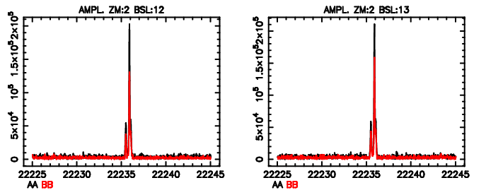
The CABB 64MHz mode.
These plots show a 20MHz chunk of the 64MHz band around the water maser in
G13.87+0.28. Click on the image for the spectra on more baselines.
Spectra from observations on 02 September 2010
(courtesy Warwick Wilson and Dick Ferris).
In its first implementation, the 64MHz mode was available as a single
64MHz band in each IF, with 2048 zoom channels across that band.
From September 2012, up to 16 zooms per IF were available.
Zoom modes
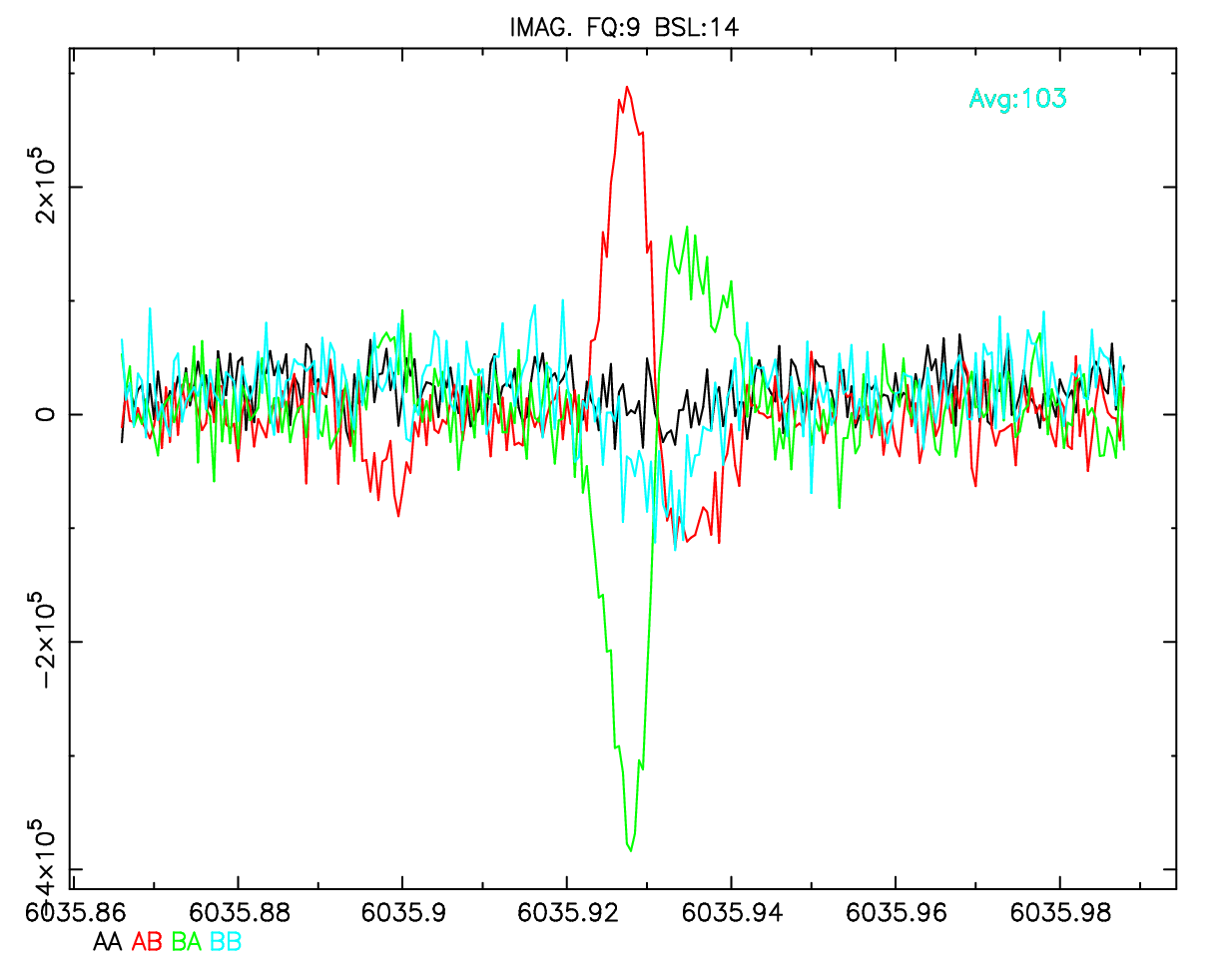
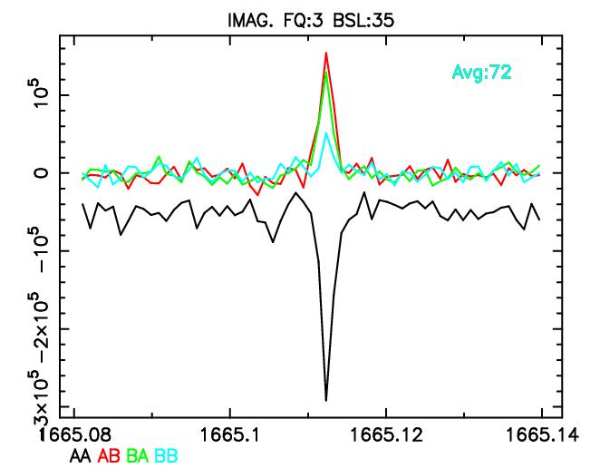
Zoom modes. (Left) A single baseline zoom spectrum,
with 2048 channels across the 1MHz bandwidth, of a methanol maser.
(Right)
CABB spectrum of excited OH at the 6035-MHz transition (the well-known
maser OH300.969+1.148). The imaginary part of the cross polarization is
plotted and reveals strong adjacent features of opposite circular
polarization (a Zeeman pair), plus another weak feature (near 6035.9MHz
on the plot) of just right-hand circular polarization .
It remains similar to the published observation of this source taken
nearly 10 years ago with the Parkes telescope (Caswell 2003 MNRAS 341,
551).
Click on an image for a higher-resolution version.
Spectra from
observations on 25 March 2010
(courtesy Warwick Wilson, Dick Ferris, Jim Caswell).
CABB was installed in March/April 2009. Initially, a single mode was available for general observing, with two 2.048 GHz bandwidths and 2048 channels across each band, corresponding to a 1 MHz spectral resolution. (In addition, a mode with a single 64 MHz channel was available for VLBI and NASA tracking.)
A discussion forum (moved in May 2011 to a new URL) has been set up for observers to discuss matters relating to CABB observing and data reduction.
Zoom mode implementation proved to take longer than first anticipated. The development of channel selection, finite impulse response (FIR) filtering and FFT has been problematic, and data transport issues have also contributed to the delay. The first 1MHz-mode zoom observations were made in May 2010.
It was decided to proceed with the development of the 64 MHz CABB mode next. This was initially implemented as a single 64MHz band in each IF, with 2048 zoom channels across the band, but restrictions on which channels could be selected for the zoom band. From September 2012, up to 16 zooms per IF were available. (There are the regular 32 channels and also the 32 interleaved channels -- offset by 32MHz in the 64MHz mode -- and the zoom channels can be placed in any of these.)

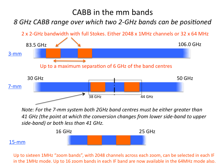
A schematic illustration of the CABB configurations in the ATCA receiver bands. The blue bars correspond to the frequency coverage of each receiver band. The orange bars correspond to the CABB 2 GHz bands. There are two CABB bands available. See the figure below for details of zoom modes. Click on image for full-resolution version.
Observers are reminded that, although correlator cycle times as short as 1 second can be used with the ATCA is special circumstances, the use of the default cycle time of 10 seconds is recommended. In the centimetre bands, the averaging option can still be used (with a default of 3 cycles) to minimise the size of output data-files. One exception is mosaic-ing observations, for which a shorter cycle time may be contemplated; however, please read the Current Issues page for the most recent information for recommended cycle times in mosaic observing.

Illustration of the CABB zoom mode. CABB internally computes two interleaved bands each of 2048 channels, and in the 1MHz mode up to 16 zoom bands may be selected (in addition to the 2048 channels across 2.048 GHz). The interleaved channels, with half-channel offsets, allow flexibility in the positioning of zoom bands so that spectral lines do not fall at a channel edge. Overlapping (interleaved) zooms are output as a single consolidated zoom. Concatenated zooms (without the overlapping interleaved band) are output as individual zoom bands. Click on image for full-resolution version.
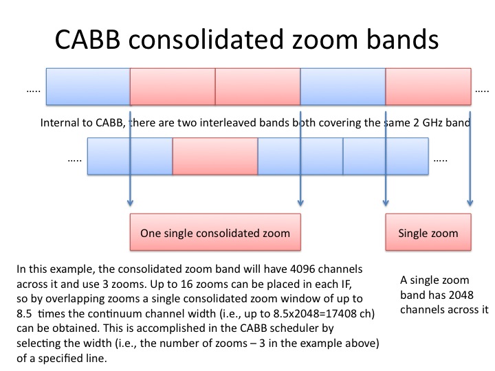
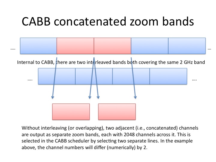

Further description of the CABB zoom modes, indicating that the zooms can be interleaved (or overlapped) to produce a single consolidated zoom band, or concatenated (i.e., abutted) or separated, producing separate output zoom bands. Click on each image for a higher-resolution version.
An overview of CABB specifications
The basic 2-GHz spectrum
A spectrum over a full 2GHz is ALWAYS observed and recorded (strictly, 2.048GHz, since all BWs and frequency separations in this document are precisely 2^n x 1-MHz). All 4 polarization products are computed. Auto-correlations are routinely computed as well as the interferometer output. Note that the 2-GHz band edges are defined by an analogue filter (as with the bands of the previous [1998-2009] ATCA correlator), so a region of roughly 32MHz at the edges of the band should not normally be used.
For this basic 2-GHz spectrum, the maximum resolution is with channels of width 1 MHz; each channel has a 'square' response and thus there are 2048 independent channels across the full spectrum. The basic 2-GHz spectrum alternatively provides 32x64MHz channels, with 128x16MHz and 512x4MHz under development. The square response prevents leakage of interference from one channel into another. Because the channel shapes are square (with no ringing) Hanning smoothing which is often used to remove ringing, will not be needed. Internal to the correlator, an output of 4096 channels is routinely computed (i.e., with additional channels interleaved with a half-channel shift) so as to allow flexibility in positioning of zoom bands (see below).
The zoom bands
Zoom bands are available in addition to the 2-GHz spectrum. Within the 2-GHz band, there are available, simultaneously, 16 zoom bands. This is the case for both the 1MHz and 64 MHz modes. If you wish to use a zoom mode, you will need to consider the alternative outputs from the basic 2-GHz band, in order to accommodate your preferred zoom mode. There will, in time, be four configurations:
- CFB 1M-0.5k: coarse resolution 1 MHz, fine resolution 0.5 kHz, (available from December 2010)
- CFB 4M-2k: coarse resolution 4 MHz, fine resolution 2 kHz, (not yet available)
- CFB 16M-8k: coarse resolution 16 MHz, fine resolution 8 kHz, (currently under development)
- CFB 64M-32k: coarse resolution 64 MHz, fine resolution 32 kHz, (available from September 2012)
In each zoom band, the output will always be 2048 independent non-overlapping channels. Interleaved channels are not computed, but the channels will ultimately be clean 'square' channels, with negligible spillage (no ringing from narrow lines and thus Hanning smoothing will not be necessary to reduce ringing). At present, the zoom channels have a (sin(Nx)/Nsin(x))2, or approximately (sin(x)/x)2, frequency response, i.e. 4.7% first sidelobe and full width half maximum 0.89 of the channel spacing. As described above, the zoom bands will ultimately have a choice of 4 widths: 1MHz, 4MHz, 16MHz, 64MHz. Each of the 16 zoom bands MUST be the width of the channel width selected for the basic 2-GHz spectrum.
The separation of selected zoom bands within the 2-GHz band can be any integral multiple of half the zoom band width. Subject to this single constraint, we can distribute them over the 2-GHz band any way that we wish. In particular, we can have an overlapping bunch at each of several different parts of the 2-GHz spectrum (see figures above). (In the overlap region of overlapping zooms, the output from the spectrometer is now seamless and does not need further blending by the user, however that was not the case initially.)
Zoom channels are specified in the CABB scheduler. Some preliminary advice on how to select zoom modes follows. The CABB scheduler now implements most of these calculations automatically, however it is still useful to understand the processes described below.
How to choose your CABB correlator configurations
If you calculate your desired spectral resolution (=channel separation in view of the square spectral response), and it is 1 MHz or more, then you do not even need the zooms. This may be the case for much continuum work, and even for extragalactic 3-mm spectroscopy.
If 1-MHz resolution is not adequate, then you investigate which zoom width (with 2048 channels) will just achieve the desired resolution. You then decide how much contiguous frequency coverage is needed, and thus how many overlapping zoom bands are needed. If you need less than 16, then there are spare zoom bands to do additional science.
Some specific examples
Example 1. Consider OH observations at frequencies of 1665.4018, 1667.359, 1720.530 MHz, 1612.231 and HI at 1420.4058 MHz, Suppose we require for each transition a frequency resolution of 0.5 kHz (to study narrowband maser emission and narrow HI absorption) and velocity coverage of about 180 km/s corresponding to 1 MHz. This combination of coverage and resolution is provided by each zoom of the CFB 1M-0.5k configuration.
All lines lie within 2 GHz. Good.
You can specify up to 16 zoom channels per IF, so it is possible to view all our lines in each IF. Since the correlator can sometimes drop blocks and thus corrupt data, you may wish to specify the same zoom configuration in each IF and thus provide a measure of insurance for such an event.
Settings for the centre frequency at each IF are constrained to integer MHz and, although not fundamental, this is likely to remain so. Note that at 16cm, the receiver sensitivity degrades quickly outside the recommended frequency range of 1.1 - 3.1 GHz. We therefore recommend that all 16cm observations use a centre frequency of 2.1 GHz (2100 MHz).
Note that even though there are several channels in the continuum bands that are missing (channels 513, 1025, 1537 and the birdie channels), you may select these channels as zoom bands with no negative consequences.
In the new sched, after specifying in 'freq1 setup' the desired freq 1 of 2100 MHz, you will notice that, if this is selected as a line frequency, its channel number is now labelled 2049, not 1025. 2049 is the centre channel of the 4096 channel centres spaced at 0.5-MHz intervals which are available for fine positioning of the zooms (and allowing concatenation of adjacent zooms). So the selected line must now not correspond to ch 2049.
We use the velocity calculator to see which frequency we prefer to centre our first line and, as an example, suppose this to be 1665.4 MHz. Entering this for line 1 will round it to 1665.5 MHz and show that the appropriate channel for the zoom centre is 2918. A width of one zoom will be adequate, with only a small shift of centre velocity (by 18 km/s) from the desired one. Entering 1667.4 and 1720.5 will show appropriate zoom channels for these two transitions of 2914 and 2808. Note that in this band the frequency decreases with increasing channel number. The scheduler takes these spectral inversions into account. If we desire a 4th zoom centre at 1612.23 MHz it will be rounded to 1612.0 or 1612.5 and a single zoom of 1-MHz will not be well-centred, so we may find the velocity coverage is not adequate and require 2 adjacent zooms. Enter 1612.23 as the line frequency and rounding will show 1612 is at channel 3025. 1612.5 is at ch 3024. If we choose a width of 2 zooms, the channels will be 3024 and 3025 and the output will be centred at 1612.25 and cover 1.5 MHz giving vel width 279 km/s in a single seamless spectrum. The scheduler will always try to get the center of the concatenated spectrum as close as possible to the sky frequency of the line. You may see the channel number jump by 1 when switching from odd to even zoom width and vice versa. You can specify the sky frequency using the built in velocity calculator or by typing it into the line frequency box for the appropriate zoom. The number displayed will be rounded to the nearest possible spectrum centre, but internally kept at full precision.
We can now choose another line fequency, e.g 1420.4058 and can decide whether the rounded frequency gives velocity coverage sufficiently well centred, or prefer a width of 2 zooms, where the centre frequency of the combination is 1420.25MHz.
Example 2 (for multiple 64 MHz zooms). Consider the 7-mm case to mimic observations reported in ATNF newsletter #62, 2007June, page 16, which were made by Maxim Voronkov with the current (pre-CABB) correlator and used a channel separation of 64kHz (i.e., 256 channels across 16MHz and thus strictly 64/1.024 kHz).
With CABB, we can use zoom bands of 64 MHz which will give us channel separation of ~32 kHz. This is a factor of 2 better than we need, but is the nearest one available.
If we want to cover as large a contiguous band as possible for a line search, we set the 16 zoom bands to overlap, and achieve a coverage of 8.5x64 MHz = 512 (+32) MHz.
We thus need 4 observations to cover the 2-GHz band.
For comparison, with the old correlator, a 2.5-GHz band was covered with 96 observations (making use of both IFs) and had spectral resolution worse than CABB by a factor of 2.
In this simple case, we estimate that CABB is faster by a factor of at least 19 for a single IF, and a factor of 38 for 2 IFs.
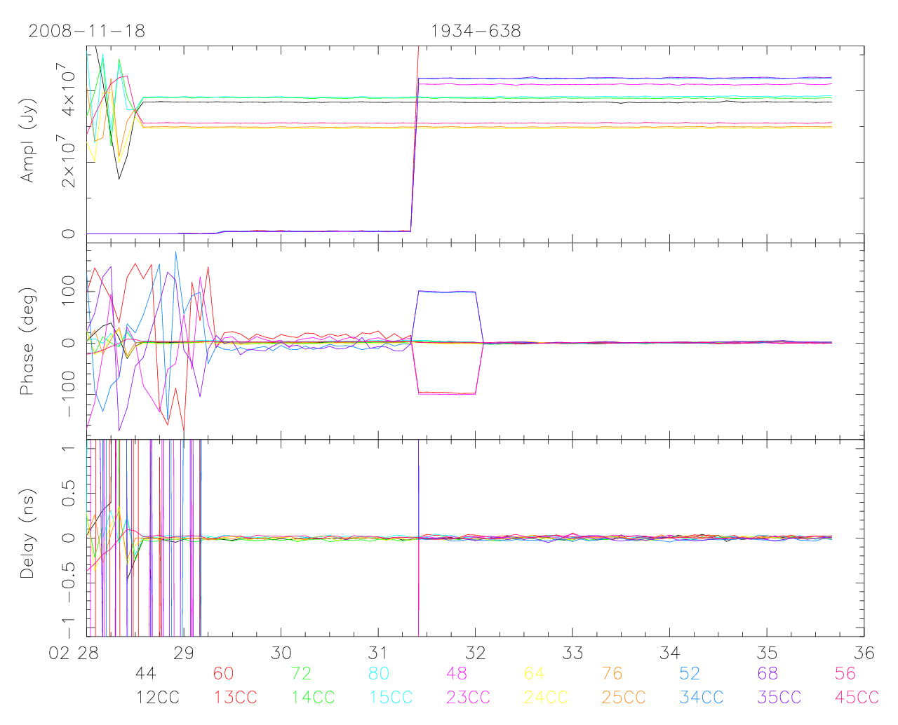
First five-antenna CABB cross-correlation! Click on image for full "vis" plot (but note amplitudes are not scaled). This observation, on 18 November 2008, used a single 128 MHz bandwidth IF, dual polarisation, in the 20cm band (courtesy Warwick Wilson).
CABB Milestones
First fringes with the interim CABB system were obtained on 23 May 2008 between CA02 and CA03. On 12 August 2008, a three-baseline system was first demonstrated with the addition of CA05, with fringes obtained on a single polarisation with a 128 MHz bandwidth, enabling further testing to be carried out. In early November, full 2GHz autocorrelation spectra were being obtained from CA01 to CA05. In early December, the first CABB image was obtained (5 antennas, single IF, 128 MHz bandwidth, full polarisation). Comparison with data from the existing correlator indicated the CABB system was working well. In late December 2008 and early January 2009, the CABB bandwidth was gradually being increased toward the full 2 GHz, with additional imaging observations being made to test the flow of data from the correlator and through miriad. In February 2009, the first observations utilising the full 2048 channels were made with the interim CABB system (five antennas, single IF). On 23 February, CA06 was taken off-line and preparations started for the full CABB installation. A six-week shutdown for the full CABB installation ran from March 2nd to April 14, 2009, and be followed by a week of scientific commissioning, with scheduled observing starting on April 22. The CABB shutdown diary provides updates on progress with the CABB installation. CABB fringes were progressively obtained to more antennas as the shutdown proceeded, with first CABB fringes to all six antennas obtained on April 1st.
Emails sent to ATCA PIs for this the first CABB semester, 2009APR, on March 31st and on April 27th with more details about observing with the new system.
The 2009APR semester was the first to offer the full 2-GHz CABB bandwidth in both frequency bands and on all six antennas. Due to the staged implementation of CABB modes, the 2009APR semester for the ATCA ran from April 22 to July 15. For 2009APRS, a single mode was available: this has 2.048 GHz bandwidths with 2048 channels across each band, corresponding to a 1 MHz spectral resolution. Proposals not completely scheduled in the 2009APR semester had to be resubmitted for consideration in the 2009JUL semester.
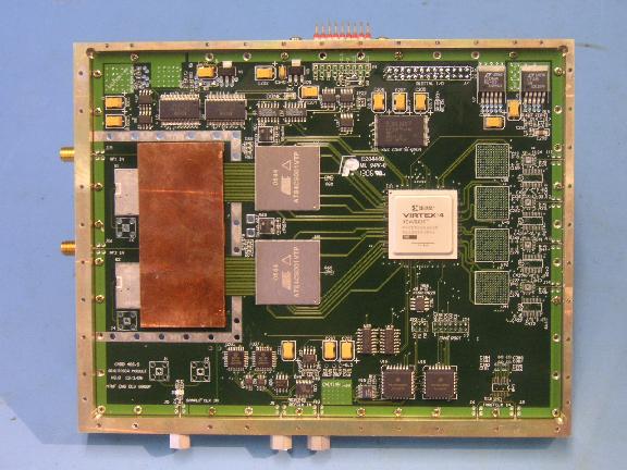
CABB ADC/data transmitter board. (Photo: Paul Roberts)
CABB hardware
The CABB project can be broadly divided into four parts: a wideband conversion system, wideband sampling, wideband optical data transmission and a complementary wideband filterbank/correlator. An overview of the sampling and data transmission is given in a February 2007 ATNF News article. The filterbank/correlator is outlined in an October 2006 ATNF News article. A description of the CABB upgrade is given in a paper by Ferris & Wilson (though note some details have changed in the final implementation of CABB). The reference to this paper is Ferris, R.H., & Wilson, W.E., 2002 URSI XXVIIth General Assembly, poster 1629.
Progress towards zoom modes: a single baseline partial zoom spectrum of the maser OH213.705 from observations on 4 March 2010 (courtesy Warwick Wilson, Dick Ferris, Jim Caswell).
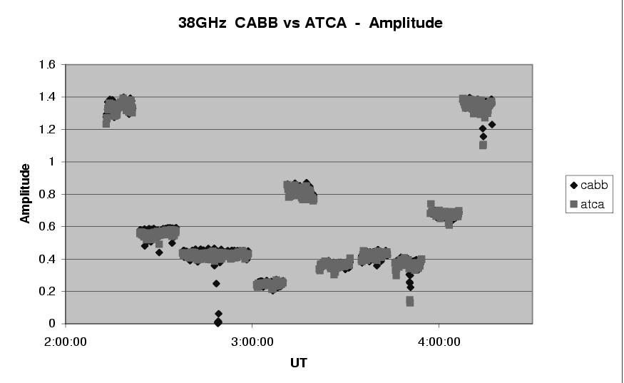
Comparison of CABB data with the existing ATCA correlator on the CA02--CA03 baseline showing the amplitudes: phase shows similarly good agreement. May 2008 (courtesy Warwick Wilson).
CABB autocorrelation spectra from antennas CA01 and CA05, November 2007 (courtesy Warwick Wilson).
CABB autocorrelation spectrum from antenna CA05 spanning 2GHz, November 2007 (courtesy Warwick Wilson).
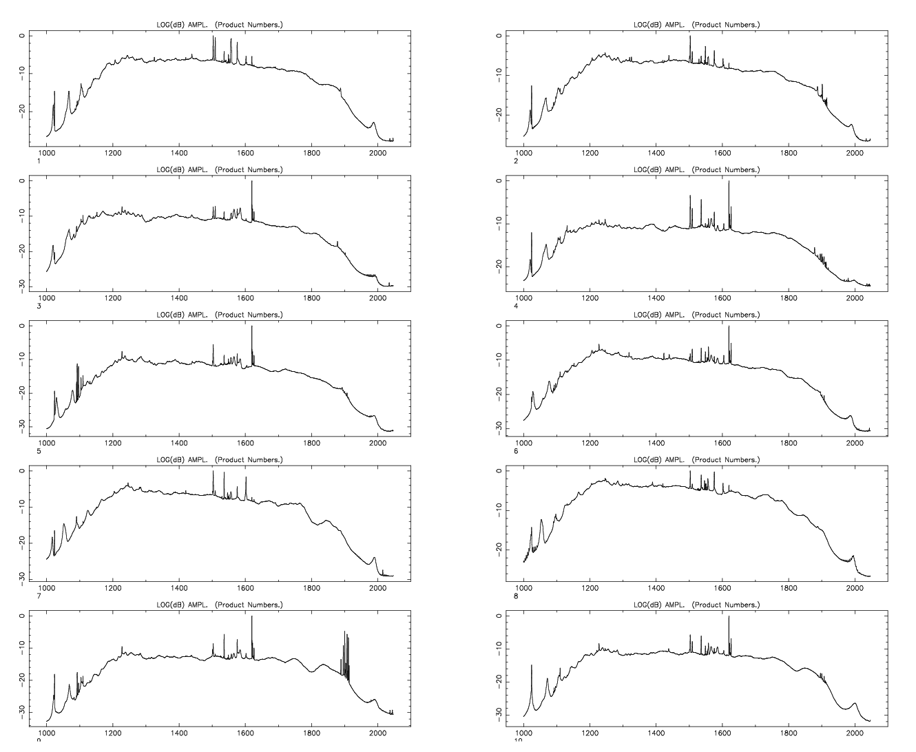
Autocorrelation spectrum of one polarization from CA01 showing the instantaneous 1GHz bandwidth of the 20cm spectrum. Click on the image to see dual-pol CABB autocorrelation spectra for CA01 to CA05. November 2008 (courtesy Warwick Wilson).
Modified: Phil Edwards (15-nov-2018)
Contributors: Jim Caswell, Dick Ferris, Dave McConnell, Warwick Wilson, Mark Wieringa, Kate Brooks, Jessica Chapman
Original: Phil Edwards (30-Oct-2007)