| Revision History | ||
|---|---|---|
| Revision 1.10 | 2022 Apr 20 | jbs |
| Add a figure to illustrate how to reboot CABB block to chapter 3. | ||
| Revision 1.9 | 2021 Nov 12 | jbs |
| Fix incorrect description of how to set noise diode periods in the caobs command list. | ||
| Revision 1.8 | 2021 Oct 20 | jbs |
| Considerable updates to all chapters to clarify some inaccuracies, and to update broken links and make HTTPS links by default, and update out-of-date information. | ||
| Revision 1.7 | 2018 Mar 15 | jbs |
| Changes recommended by ATUC, including clarification of NAPA/ToO policies, and of what is expected during unattended observing. | ||
| Revision 1.6 | 2017 Jun 01 | jbs |
| Changes relating to the rapid response mode | ||
| Revision 1.5 | 2016 Sep 14 | jbs |
| Changes relating to the RFI surveys at 4cm and 15mm | ||
| Revision 1.4 | 2016 May 31 | jbs |
| Changes relating to the ATCA alarm Twitter feed | ||
| Revision 1.3 | 2016 May 9 | jbs |
| Changes relating to the new 1934-638 high-frequency flux density scale | ||
| Revision 1.2 | 2016 Apr 26 | jbs |
| Revert a change after a fix to vis | ||
| Revision 1.1 | 2016 Apr 21 | jbs |
| Add a section that can be updated with the latest changes | ||
| Revision 1.0 | 2014 May 31 | jbs |
| Initial Docbook revision | ||
This manual describes how to apply for observing time, make a schedule file, and carry out an observation with the Australia Telescope Compact Array (ATCA).
This manual is a reference guide: you do not need to read all of it to use the ATCA. Chapter 1 describes the telescope and what you need to know before proposing to use it. Chapter 2 can be read after getting observing time on the ATCA. It describes how to prepare for your observations. Chapter 3 deals with the online software and all the details of how to actually do your observations. Chapter 4 goes into detail about what to do with your data after it has been collected. The appendices provide additional details above and beyond what will usually be required for routine observing.
In 2014 April there was a major overhaul of this manual: the presentation of the document on the web and in print was improved, and the content was significantly updated. Copies of this manual and other ATNF documentation can be obtained from the ATNF webpages.
If you find that any part of the Compact Array doesn't work as described
in any of our documentation, please email the ATCA Users Guide (ATUG)
editorial team at <atca_userguide@atnf.csiro.au>, or start a conversation at the
ATCA Forum.
Comments on documentation are especially welcomed.
If you can't find the information you require in this Users Guide and would like to ask our expert users how to do something, please visit the ATCA Forum website.You can also start or participate in conversations about your experiences with the ATCA, as well as find out about any issues that can affect your data and how to deal with them.
If you are completely new to radio interferometry, the following reading is recommended:
Remind yourself about Fourier theory — an appropriate summary can be found in Chapter 1 of Bracewell (1978, 1986, 1999).
Review the principles and techniques of radio-astronomy, e.g., Kraus (1986); Christiansen & Hogbom (1985); Thompson, Moran & Swenson (1986, 2001). The latter is probably the best single book on the subject of radio interferometry.
Read the introductory chapters of one of the NRAO Synthesis Imaging Summer School lectures in Perley, Schwab & Bridle (1989) or Taylor, Carilli & Perley (1999).
Perhaps also look at Galactic and Extragalactic Radioastronomy by Verschuur & Kellermann (1988) if you are not already familiar with the field.
The latest changes to this manual were made on April 20 2022.
- Re-add a slighly modified flowchart to show how to reboot a CABB block ???.
Changes to this manual were made on October 20 2021.
- New contributors!
- Broken links were fixed or removed, and links were made HTTPS unless not possible. Links to out-of-date separate web pages were removed.
- Update due to change of name to Space & Astronomy.
- Remove references to Friends, which are no longer offered.
- Clarify how the array works when tracking non-sidereal sources.
- Table 1.3 was updated for upcoming semesters.
- Remove CABB modes that are never coming from Section 1.4.3.
- Update Figure 1.3 for the new 4cm feedhorns, and improved axis labels.
- Update Figure 1.4 with RFI survey from 2018.
- Update Table 2.2 to include advice about when to use (or not) the 15mm recommended frequencies to avoid SkyMuster RFI.
- Add a new flowchart for problem solving when no correlation is observed in Section 3.5.6.
- Update Section 3.6.3.3 to remove references to the SMS service that Twitter no longer offers.
- Update information in Section 4.1.3 to show how to access data now that kaputar has been turned off.
- Updated information on how to properly acknowledge ATCA in publications in Section 4.4.
Changes to this manual were made on March 15 2018.
- Policies around how NAPA and ToO requests are considered, including for the rapid response mode, are now described in Section 1.11.2.
- A description of what is expected of observers when they choose to operate in “unattended observing” mode, and the tools available to help them do so, is now available in Section 3.6.
Changes to this manual were made on June 1 2017.
- Section 2.5 was created to document the new rapid response mode.
Changes to this manual were made on September 14 2016.
- Section 1.3.2 was updated to show the results of recent 4cm and 15mm RFI surveys.
- The recommended CABB continuum central frequencies in the 15mm band were changed in Section 1.3 to avoid RFI from the “Sky Muster” satellite.
- Table 1.3 was updated for upcoming semesters.
Changes to this manual were made on May 31 2016.
- Section 3.6.3 was created to describe how to use the ATCA alarm Twitter feed to get notifications of problems while not at your computer.
Changes to this manual were made on May 9 2016.
- Section 2.2.4 was updated to show the new high-frequency flux density scale based on 1934-638, derived from quasi-simultaneous observations of calibration sources with ATCA, VLA and Planck.
- Table 2.3 was updated to indicate that 1934-638 is now the preferred flux density calibrator for 7mm observations.
- Describe how the Miriad flux density scale changed in May 2016 to use the new 1934-638 high-frequency model, and how to switch back to the old model if required, in Section 4.3.2.6.3.2.
In this manual we use some typographical conventions to help clarify the documentation.
Computer system names, e.g. xbones
Software packages, e.g. Miriad
Software program, e.g. caobs
Command example, e.g.
$ df -h
Filename, e.g.
output.txtProgram option, e.g.
rfiflagParameter name, e.g.
edgeAstronomy-related acronym, e.g. USB (upper sideband)
Non-astronomy-related acronym, e.g. USB (universal serial bus)
Placeholder for changeable parameter, e.g.
ca0#Optional parameter, e.g.
[ca0#]List of potential commands or parameters, e.g.
disable|enable. These might also be wrapped in curly brackets, e.g.{ca0#|default}
Table of Contents
- Preface
- 1. The Australia Telescope Compact Array
- 1.1. The Australia Telescope National Facility
- 1.2. Overview of the ATCA
- 1.3. Choosing an Observing Frequency
- 1.4. Choosing Angular and Frequency Resolution
- 1.5. Centimetre Observations (16–4 cm bands)
- 1.6. Millimetre-wave observations (15mm–3mm)
- 1.7. Additional Observing Notes and Techniques
- 1.8. High Time Resolution, Pulsars, Planets and VLBI
- 1.9. Other Things to Consider
- 1.10. Submitting a proposal
- 1.11. Successful Proposals and Observing
- 2. Preparing for Observations
- 2.1. Observational Sensitivity
- 2.2. Calibration
- 2.2.1. What type of calibration do I need to do?
- 2.2.2. What sources can be used for delay calibration?
- 2.2.3. How do I calibrate the bandpass response of the antennas?
- 2.2.4. How do I calibrate the flux density of my observations?
- 2.2.5. How do I best calibrate the time-varying gains?
- 2.2.6. What do I need to do for polarisation calibration?
- 2.2.7. When is pointing calibration required?
- 2.2.8. When is paddle calibration required?
- 2.3. Scheduling your observations
- 2.3.1. What is meant by “schedule”?
- 2.3.2. How do I best observe if I want to image compact sources?
- 2.3.3. How do I best image a source with a large angular extent, or a wide field region?
- 2.3.4. How do I schedule a mosaic observation?
- 2.3.5. How do I best map regions of spectral line emission?
- 2.3.6. Are there limits to the frequencies I can observe?
- 2.3.7. Can I change between frequencies during my observations?
- 2.3.8. How do I observe a planet in our Solar System?
- 2.3.9. How do I observe a minor object in our Solar System?
- 2.3.10. What are the antenna “wraps”?
- 2.3.11. How do I prepare a schedule file?
- 2.3.12. Could I see an example continuum schedule file?
- 2.3.13. Could I see an example spectral-line schedule file?
- 2.4. Running a schedule
- 2.5. Rapid Response Mode
- 2.5.1. Who can use the rapid response mode?
- 2.5.2. How does the rapid response mode work?
- 2.5.3. Can I over-ride any scheduled block?
- 2.5.4. How can I make a schedule file automatically?
- 2.5.5. What is this authorisation token that I need?
- 2.5.6. But how do I make a request?
- 2.5.7. How can I find out what the service is doing?
- 2.5.8. What is the recommended strategy for a rapid response schedule?
- 2.5.9. How does the service shorten my schedule?
- 2.6. Pre-observation Checklist
- 3. Observing
- 4. After your Observations
- A. caobs reference
- B. cacor reference
- B.1. cacor Status Panel
- B.2. cacor Data Panel
- B.3. cacor Timing Panel
- B.4. cacor Log Panel
- B.5. cacor Command Panel
- B.6. cacor Commands
- B.7. Changing Correlator Configs
- B.8. Changing to 1MHz, No Zooms
- B.9. Changing to 64MHz Zooms
- B.10. Changing to Hybrid Config (1MHz Continuum and 64MHz Zoom Mode)
- B.11. Changing to Pulsar Binned mode
- B.12. Changing to 1MHz Zooms
- B.13. CABB issues
- C. SPD reference
- D. vis
- E. MoniCA
- F. Web Scheduler
- G. Observatory Coordinates
- H. ATCA Configurations
- Index
| Revision History | ||
|---|---|---|
| Revision 1.6 | 2021 Oct 8 | jbs |
| Change links to HTTPS where possible, and fix broken links. Update information regarding recent change of name to Space & Astronomy. Fix the incorrect noise-diode injection rate and the Tsys equation. Remove confusing wording regarding conversion band simultaneity. Update the Tsys and 16cm RFI survey plots. Update the config table for future semesters. Remove CABB modes that are never coming. Clarify tracking of non-sidereal objects. Remove information about friends. Other minor clarifications throughout. | ||
| Revision 1.5 | 2018 Mar 15 | jbs |
| Clarified the rules and procedures around NAPA and ToO requests, and how time is allocated to them. | ||
| Revision 1.4 | 2016 Sep 14 | jbs |
| Added discussion of the 4cm and 15mm RFI we now know about, and change the 15mm recommended continuum frequencies. Update the upcoming configurations table. | ||
| Revision 1.3 | 2015 Nov 20 | jbs |
| Added discussion of the 16cm RFI environment, RFI monitor and mid-week RFI | ||
| Revision 1.2 | 2015 Oct 20 | jbs |
| Updated information about observing at the SOC | ||
| Revision 1.1 | 2014 May 30 | jbs |
| Revised out-of-date tables and figures | ||
| Revision 1.0 | 2014 Mar 20 | jbs |
| Initial Docbook revision | ||
This chapter gives an overview of the Australia Telescope Compact Array (ATCA) and provides the information needed to prepare an observing proposal. The old Users Guide is still available and is recommended for those reducing pre-CABB data (i.e., observations before April 2009).
The ATCA consists of six 22-m radio antennas which can be configured with antenna spacings of up to 6km, located at the Paul Wild Observatory near Narrabri, some 550 km northwest of Sydney. It is one of the telescopes operated by the Australia Telescope National Facility (ATNF).
The ATNF is managed as a National Facility by the Commonwealth Scientific and Industrial Research Organisation (CSIRO). Formerly part of the CSIRO Division of Radiophysics, it became a separate division in January 1989. The ATNF became a National Facility in April 1990. In December 2009, ATNF became part of a new Division, CSIRO Astronomy and Space Science (CASS), together with NASA Operations (including the Canberra Deep Space Communication Complex), and CSIRO Space Sciences and Technology. In May 2021, the division name changed to CSIRO Space and Astronomy (S\&A). The Australia Telescope continues as a National Facility, providing world-class observing facilities for astronomers at Australian and overseas institutions.
The ATNF employs about 185 staff, including about 40 astronomers, with the majority of staff located at its headquarters in Marsfield, a suburb of Sydney (although Marsfield is sometimes referred to as Epping, a larger neighbouring suburb). The site was shared with the AAO (the Australian Astronomical Observatory, or before 2010, the Anglo-Australian Observatory) until 2012, when the AAO relocated to the nearby suburb of North Ryde.
Besides the ATCA, the ATNF operates the 64-m radio telescope at the Parkes Observatory (300 km west of Sydney). The ATNF negotiates time with the CSIRO-administered 70-m and 34-m antennas at the Tidbinbilla Deep Space Tracking station outside Canberra. The ATNF telescopes are used together, in conjunction with the University of Tasmania telescopes at Hobart and Ceduna, and the Auckland University of Technology antennas at Warkworth, as part of the Long Baseline Array for Very Long Baseline Interferometry (VLBI) observations. .
ATNF scientists and engineers also operate ASKAP (the Australian SKA Pathfinder telescope) located 300km inland from Geralton in Western Australia. ASKAP is an array of thirty-six wide-field 12m antennas. operating in the 0.7–1.8 GHz range. More details are available at the ASKAP project website.
The ATCA is an array of six 22m diameter antennas located 237m above sea level at latitude -30° 18′ 46.385″ south, longitude 149° 33′ 00.500″ east. The array has a 3km east-west track with a 214m northern spur. Five antennas can be moved along these tracks, with the sixth antenna at a fixed position 3km to the west of the east-west track. The longest possible baseline is, therefore, 6km. The array can be used for observations in five wavelength bands between 27cm and (with five antennas only) 3mm, between frequencies of approximately 1.1GHz and 105GHz.
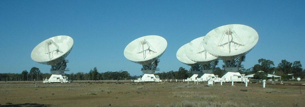
The location of six antennas at six stations is called an array configuration, or often, simply a configuration. The westernmost antenna, CA06, is fixed in position. The other five antennas can be positioned at any of 44 fixed stations. The station posts provide mains power to the antennas and network connections that allow commands from the control building to be sent to the antenna, and monitor data to be received from the antenna. The posts also have high-speed optical links that allow data from the antenna to be transferred to the control building. The smallest baseline increment available is 15.306m, and the shortest physical baseline is 30.612m. Five of the six ATCA antennas are shown in Figure 1.1.
A standard set of 17 configurations has been defined, and a subset of these is offered for each semester. These configurations have been designed to give optimum, minimum-redundancy coverage after a 12 hour observing period. Four configuration sets for the principal arrays (750m, 1.5km and 6km) are offered over several semesters (see Appendix H for details of these sets). Your choice of configuration depends on the extent, brightness and complexity of your source (see below).
The Australia Telescope Compact Array is an earth-rotation aperture synthesis radio interferometer. Earth-rotation aperture synthesis was first used in the 1950s for radio observations of the sun. The technique is comprehensively explained, with a historical perspective, in Interferometry and Synthesis in Radio Astronomy by Thompson, Moran & Swenson (Wiley, 3rd edition, 2017). Essentially, the array of antennas is comprised of a number of two-element interferometers. The visibility (i.e., the fraction of the signal common to both antennas of a pair) is derived by multiplying the (suitably delayed) signals together. By combining the correlated signals obtained over a long period of time and with a large range of spacings between antennas, the Compact Array measures the spatial coherence function:
where is the two dimensional intensity distribution on the sky, is the unit vector in the direction of the celestial source, is the separation vector between antennas 1 and 2 and indicates integration over the sphere (or, in practice, solid angle of the antenna beam).
The van Cittert–Zernike theorem states that the Fourier transformation of the spatial coherence function yields the source brightness distribution, i.e., the Fourier Transform of the visibilities produces an image of a radio source. The image is formed with the same angular resolution as for observations with a single antenna with a diameter equal to the largest spacing, however it will be less sensitive due to the interferometer's smaller collecting area.
By plotting the tracks that the baseline vectors trace out (from the source's perspective) as the Earth rotates, astronomers can gauge how good the telescope will be at imaging the source and resolving components in the field of view. This plot is referred to as the (u,v)-coverage as, by convention, the two orthogonal axes of the plot are u and v. These variables have units of the observing wavelength. The (u,v)-coverage shows where on the Fourier plane the image has been sampled.
To obtain the fullest (u,v) coverage with the ATCA would require observations with multiple different configurations, and for twelve hours with each configuration. However, almost any program can be successfully carried out with less than complete (u,v) coverage, and the individual configurations are chosen so as to optimise single configuration imaging characteristics. Sophisticated off-line image processing techniques minimise the effect of missing (u,v) coverage and allow reasonable images to be made with one configuration. For most programs, one to four configurations provide the best compromise between dynamic range, (u,v) coverage and time.
The smallest synthesized beamwidths in Right Ascension for each observing wavelength are shown in Table 1.1, but bear in mind that, for east-west arrays, the beamwidth in Declination is greater by a factor cosec(Dec). At high angular resolution, the telescope is only useful for observing southern objects. North of Declination -24°, full (u,v)-coverage is unobtainable; near Declination zero the beam is highly elongated north-south; and north of Declination +48° sources are below the telescope's +12° elevation limit and are inaccessible. For lower angular resolution, the north-south and hybrid arrays improve the (u,v)-coverage for equatorial sources, but only up to a maximum north-south baseline of 214m.
The rest of this chapter outlines the structure and operation of the ATCA. The path of the radio signal is traced through the system from the dish to the final data recording. This section is designed to help you understand how the Compact Array operates and provide all the information required to design an appropriate experiment. Detailed technical information about the ATCA can be found in the Journal of Electrical and Electronics Engineering, Australia, Special Issue, Vol. 12, No. 2, June 1992, a copy of which is available in the control room at the Narrabri Observatory.
The antennas have a Cassegrain design, i.e., the receivers are located in a turret that protrudes through the main reflector surface — see Figure 1.1. The antennas have an altitude-azimuth mount with wrap limits as shown in Figure 2.1. The shaped (i.e., non-parabolic) dish and subreflector surfaces are designed to maximise the gain to antenna noise ratio. The reflecting surface of antennas 1–5 are solid panels that allow observations up to 116 GHz. This is also true of the inner 15.3m of antenna 6. The outer reflecting surface of antenna 6 is made of perforated panels which permit observations at frequencies up to 50 GHz.
The subreflector mounted near the prime focus has a specially designed shape, differing slightly from the hyperbolic secondary of standard Cassegrain optics. The feedhorns are mounted on the optic axis — this allows polarisation measurements to be made, with very low ( ) instrumental polarisation. Subreflector height can be adjusted to achieve optimal focus for the different frequency bands. A major feature of the ATCA is its wide bandwidth operation. The feedhorns and front-end electronics operate over a very large range of frequencies, thus allowing (u,v) coverage to be increased by multi-frequency synthesis and dual frequency observations. The feedhorns are compact, with a corrugated interior surface and are designed for maximum frequency coverage, low noise, low spillover, low reflection and low cross-polarisation sidelobe levels. The feedhorns allow two simultaneous orthogonal linear polarisations to be measured (at frequencies almost an octave apart), and have a main lobe with near-constant, symmetrical beamwidth (James, G.L., 1984, IEEE Trans. Antennas Propagat. AP–22, pp 1134–1138; Thomas, B.M., James, G.L., Greene, K.J., 1986, IEEE Trans. Antennas Propagat. AP-34, pp 750–757).
The frequencies at which the Australia Telescope operates are listed in Table 1.1 see also section Section 1.3.1.
Each range of frequencies is referred to as a band. Bands are referred to by the wavelength of the approximate centre of the band or (especially at higher frequencies) by the frequency (and sometimes by the letter-codes shown over the columns of Table 1.1. There are presently five feedhorns mounted on each antenna (four on antenna 6): a large (2m high) feed-horn that operates in the 16cm band, and a somewhat smaller (50cm high) 4cm band feedhorn and three (several cm high) feedhorns mounted on the same dewar for the 15mm, 7mm and 3mm wavelengths. The feedhorns and the receivers are mounted on a rotating turret. The rotating turret design ensures that all feedhorns, when brought on-axis, are aligned with the optic axis of the antenna, allowing a wide field of view and dual-polarisation observations. The turrets are rotated automatically in accordance with the frequencies selected by the observing file. Rotating the turret orients the desired feed-horn and also ensures that the subsequent electronics suit the frequency at which you are observing. Changing the observing band to or from 7mm requires first rotating the turret to the 15mm position, and then translating the whole mm dewar to bring the 7mm feed on axis. The latter stage takes 2~3 minutes, and so changes to or from 7mm are much slower than any other band change.
Both the 16cm and 4cm band feedhorns are fitted with wide-bandwidth receivers that covers the horn's entire usable frequency range. All receivers run continuously and use cooled HEMT (high electron mobility transistor) and FET (field effect transistor) amplifiers that provide wide bandwidths and total system temperatures between 20K to 65K, depending on frequency.
The signals collected by the feedhorns are fed to the receiver systems for amplification and conversion to standard intermediate frequencies. During observations each antenna provides four independent intermediate frequency (IF) outputs (two frequency bands, two polarisations). These channels allow simultaneous observations of both polarisations at the two available frequencies in either dual-receiver system. The frequencies can be anywhere in the range covered by the selected feed-horn except at 15, 7 and 3mm where the two frequencies must be less than 6 GHz apart, and not straddle the 7mm sideband inversion (see Section 2.3.6).
In order to convert the received radio signals to lower frequencies, the radio signals are mixed with a “local oscillator" signal. Four local oscillator signals provide four IF outputs to enable the dual-frequency, dual-polarisation operation. You can also switch frequencies at the end of each integration cycle (typically ten seconds). To change to a pair of frequencies covered by a different feed-horn requires a rotation of the turret and takes about twenty seconds. However, to avoid excessive wear of the turrets, a limit of four rotations per hour is imposed. Thus time sharing between a number of frequencies is limited only by signal to noise ratio, wear and tear on the equipment, your imagination, and the off-line software.
The following sections describe the path of the signal from the initial reflection off the antenna surface, through to the data recorded onto export media, in more detail than the introduction above. Some radio-astronomy jargon is also explained, as is some important mathematics. The details of this section are not required by observers, but are included for completeness. A knowledge of the system is however essential if you want to design an experiment that uses the array in a new or unconventional way. Familiarity with the names and functions of some critical components can also be helpful if you need to diagnose faults. Many system components are housed in modules, and repairs can be made quickly by local staff replacing a module once a correct diagnosis has been made.
Radio waves (approximately within a range of 300 MHz to 120 GHz) are accurately reflected from the primary surface of the main parabolic dish and are re-reflected off a secondary reflector into a feed-horn. At the base of the feed-horn is a directional, coupling waveguide. In this coupler (the noise coupler) is a diode that injects a noise signal of known amplitude. This noise signal is used to calibrate the system temperature (Equation 1.1) and gain of the receiving system.
For radiation emitted by a randomly polarised source, the power received by a radio telescope is given by:
where A is the effective area of the antenna, S is the spectral power flux density and is the range of frequencies observed (the effective bandwidth). The factor of occurs because a detector can only respond to one polarisation component of the randomly polarised wave. The ATCA overcomes this limitation by providing separate detectors and electronics for two orthogonal polarisations, thus allowing all the power in the wave to be detected.
Table 1.1. Observing Parameters for the 6km Compact Array.
| Band Name | 16cm | 4cm | 15mm | 7mm | 3mm |
|---|---|---|---|---|---|
| Band Code | L / S | C / X | K | Q | W |
| Frequency Range (GHz) | 1.1 - 3.1 | 3.9 - 11.0 | 16 - 25 | 30 - 50 | 83 - 105 |
| Fractional frequency range | 95% | 95% | 44% | 50% | 24% |
| Number of antennas | 6 | 6 | 6 | 6 | 5 |
| Number of baselines | 15 | 15 | 15 | 15 | 10 |
| Primary beam [a] | 42′ - 15′ | 12′ - 4′ | 2′ | 70″ | 30″ |
| System temperature (K) [b] | 45 | 36 | 60 | 112 | 724 |
| System sensitivity (Jy) [c] | 55 | 43 | 72 | 136 | 1051 |
| Strongest confusing source (mJy) [d] | 140 - 24 | 2.3 - 0.4 | — | — | — |
| Array assumed below | 6 km | 6 km | 6 km | 6 km | H214 |
| Synthesized beam [e] | 9″ - 3″ | 3″ - 1″ | 0.5″ | 0.2″ | 2″ |
| Bandwidth assumed below (GHz) | 2 | 2 | 2 | 2 | 2 |
| Centre frequency assumed below (GHz) | 2.1 | 7.0 | 17.0 | 40.0 | 95.0 |
| Flux sensitivity (mJy/beam) (10 min) [f] | 0.04 | 0.03 | 0.05 | 0.09 | 0.70 |
| Brightness sensitivity (K) (10 min) [g] | 0.1 | 0.1 | 0.16 | 0.29 | 0.02 |
| Flux sensitivity (μJy/beam) (12 hr) | 4 | 3 | 5 | 33 | 83 |
| Brightness sensitivity (K) (12 hr) | 0.02 | 0.01 | 0.02 | 0.01 | 0.002 |
[a] Field of view (full width at half power). [b] The system temperature at high elevation under reasonable weather conditions. These values, particularly at high frequency, are weather-dependent. [c] The signal which doubles the system temperature. [d] Within FWHM primary beam — see A.H. Bridle, in Perley R.A., Schwab F.A. & Bridle A.H. (1989) “Synthesis Imaging in Radio Astronomy” Astron. Soc. Pacific Conf. Set., 6, p.471. [e] HPBW in R.A. for the 6 km array for all bands except 3mm, for which the H214 array is assumed. No taper applied. In Declination, for the 6 km array (and other pure east-west arrays), the HPBW is larger by cosec(Dec). Longer arrays (up to 3 km) are possible at 3mm but only with self-calibration and under favourable weather conditions. [f] Theoretical rms noise; one frequency; dual orthogonal polarisation; natural weighting. The effect of confusing sources can substantially degrade this number. This is the 1σ Gaussian-noise level. [g] For the array listed in the same column: see following table for shorter arrays. This is the 1σ Gaussian-noise level. | |||||
The sensitivity of a radio telescope is the minimum signal power that can be distinguished from the random fluctuations at the output of the receiving system which are caused by noise inherent in the system. The sensitivity is usually defined as the spectral power flux density of a source that would produce the same signal power as the noise power. It is measured in Jansky (Jy), with
The noise power consists of two main components: the noise power due to the receiving amplifier and other electrical system components, and the noise due to ground radiation, thermal emission from the atmosphere (which varies with elevation, cloud cover, etc.), background radio emission from our Galaxy and other sources detected by the antenna. These noise powers are usually referred to as equivalent temperatures, although at no point is a physical temperature measured. The “temperature” due to the noise power is called the system temperature, , and is related to the noise power by:
where
is the noise power and
is Boltzmann's constant. As both the source and noise signals are random
in nature, measurements of the power levels made at time intervals
separated by
can be considered independent
(e.g., Thompson, Moran & Swenson 1986, 2001). If the signal level is
averaged for
seconds then
samples have been measured.
The signal to noise ratio is the ratio of the power in the output that is due to the radio source being observed to that caused by the noise, and is given by:
In this expression, is the antenna temperature, the equivalent temperature of the radio source being observed. Note that “antenna temperature" is sometimes also taken to mean the contribution to the noise power from radio noise detected by the antenna, as described above. For typical values for bandwidth (2 GHz) and integration time (12 hours), it is possible to detect a signal for which the power level is less than times the noise level.
The noise source in the noise coupler injects a signal that is about 5% of the level of the system temperature at a rate of 8 Hz. This noise signal is synchronously demodulated and the following relationship holds:
Here,
is the equivalent temperature of the noise
source,
is the power received while the noise diode is
on, and
is the power received while the noise diode is
off.
is measured accurately once by placing a thermal
radiator of known temperature (a microwave absorber at 300K, giving
300K
)
directly above the feeds. The power received
with this load in place is then compared with the power output with
the antenna just looking at the sky (
).
This measurement is used to establish the level of
,
which is assumed not to vary with time. The measurement of system and antenna
temperature is described in a
technical memo by
Sinclair and Gough (1991). And despite our assumption that this level should not
vary with time, it can be calibrated by the correlator at any time using a point source
with a known flux density, with the acal command
(Section 3.3.6.4).
The noise coupler is mounted on another coupler that provides a vacuum seal between the noise coupler and the subsequent receiver system, which is housed in an evacuated, cryogenic cylinder. An air gap thermally isolates the cylinder, the contents of which are cooled by a helium pump to 20K. The second coupler is mounted on the polariser. The dual function of the polariser is to select the two linear polarisations and the desired band, so it is also known as a band splitter. The polariser consists of four strips of metal inside a conical waveguide that “guide” two orthogonal linear polarisations into probes at the narrow end of the polariser. The way in which the metal strips select the linear polarisations can be thought of as analogous to the effect of a ridged waveguide, which constrains a particular mode to propagate along the region between the ridge and the roof of the waveguide. The probes are simply short (with respect to the wavelength) lengths of the cores of the coaxial cables that take the signal into the first amplifiers. Thus the polariser converts a wave into a voltage: the impedance of the circuit is effectively the same as a waveguide impedance, so it works like a well-matched load. The polariser's official title is quad-ridged orthomode transducer, or OMT. Separate electronics exist for both orthogonal linear polarisations, which are measured simultaneously. The position angle of the polariser is fixed with respect to the antenna. As the antennas have altitude-azimuth mounts, the position angle of the linear probes rotate on the sky during the course of an observation (imagine a circumpolar line on the sky orbiting around a stationary antenna). Measurement of both polarisations is therefore required for polarised sources. The two linear polarisations can be combined to give an accurate total intensity: the Stokes I parameter. Without additional calibration, the other Stokes parameters (the linear polarisation measures Q, and U, and the circularly polarised component V) can be in error by about 2% of the value of I. Measurements of the phase difference of the two linear polarisations (referred to as the X and Y (or A and B) polarisations) at the receiver by on-line hardware may need further off-line calibration.
For an unpolarised source, observing both orthogonal polarisations offers a improvement in signal to noise ratio for an I image over an image generated from only one polarisation.
The signal is taken from the feedhorn into a low noise, broadband amplifier.
The receivers each use two low-noise amplifiers (LNAs) to amplify the signal by 30–40 dB. All six antennas are fitted with wideband, continuously running, receivers. Cooled indium-phosphide high electron mobility transistors (InP HEMTs) are used at 16cm and 4cm, and indium-phosphide monolithic microwave integrated circuit (InP MMIC) devices are used at 15mm, 7mm and 3mm. Only the “inner" five antennas (i.e., excluding CA06) have 3mm receivers. The accessible frequency range is given in Table 1.1, and the average system temperatures are given in Table 1.4 and in Section 1.3.1. Note that frequencies outside these nominal limits may be accessible.
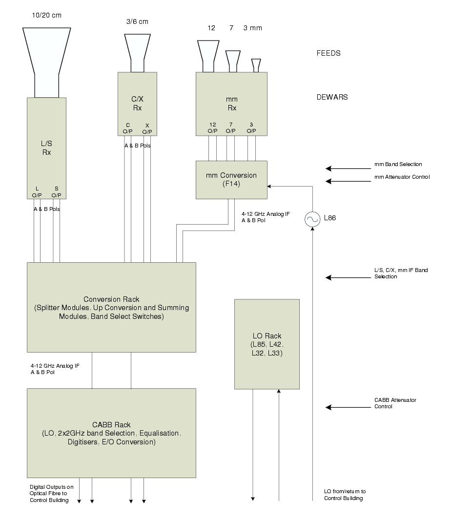
The next step is the conversion to the frequency range that is used by the CABB digitisers. The 4cm signals require no conversion, whereas the mm signals require a down-conversion stage, and the 16cm signals require up-conversion to the 4 to 12 GHz band.
The local oscillator signals have a relatively narrow tuning range, lying in the regions between the radio frequency bands (this reduces the likelihood of self-generated interference).
The final output from the conversion system is sent to the samplers for digitisation. The CABB (Compact Array Broadband Backend) samplers were developed in-house and are capable of 4 gigasamples per second (GS/s), with 10 bit sampling (more information is available in the February 2007 ATNF newsletter and in Wilson et al. (2011, MNRAS, 416, 832)).
The samplers, which are also referred to as the CABB digitisers, do two things. First the analog (continuously variable in time and amplitude) signal is sampled into a discrete-time sequence of values. This process does not degrade the signal as it is sampled at the Nyquist rate (twice the inverse frequency of the bandwidth of the analog signal). Subsequently, each of the discrete-time, continuously variable values are converted to one of a finite set of values: this is called quantising. CABB uses 9-bit sampling (internally, as stated above, 10-bit sampling is used, with 9 bits transferred to the correlator), with approximately 6-bits used in sampling the regular data range, and the additional bits providing extra robustness in the case of interference RFI (radio-frequency interference). The digitised signals from the sampler are sent from each antenna to the correlator along optic fibres at a rate of 160 gigabits per second for each antenna. Optical fibres run from the samplers in each antenna to the correlator, which is housed in the screened room (to prevent RFI generated by the correlator electronics from affecting the observations) of the central control building. Synchronising code is added to the data stream at the start of each integration cycle to allow each bit to be correctly identified at the correlator irrespective of temporal changes in the length of the fibre.
The correlator effectively multiplies simultaneous signals from two samplers: the more similar the signal from both antennas, the larger the degree of correlation. A plane wavefront approaching the ATCA will, in general, arrive at different antennas at different times. The signals from the antennas therefore need to be delayed before being presented to the correlator so as to simulate a wavefront arriving at each antenna simultaneously. This was previously achieved by separate delay units, but is now included in the CABB boards. The delay calibration undertaken at the start of an observation removes other delays caused by return path length differences, instrumental delay variations and the like, so that wavefront samples are presented to the correlator synchronously.
The CABB filterbank/correlator is divided across a number of Digital Signal Processing (DSP) boards. The DSP boards use Virtex-4 Xilinx Field Programmable Gated Arrays (FPGAs) to provide a flexible, programmable hardware correlator. The output from the correlator is averaged for the period of one integration cycle, and sent to the correlator control computer caccc where it is written to hard disk. Integration cycles can be set by the observer, between 2 and 30 seconds, although the default cycle time of 10 seconds is generally recommended for all observers. (For mosaic-mode observations, 6-seconds is the practical minimum cycle time.)
More information on the correlator can be found at the CABB webpage.
The CABB correlator provides a number of observing modes:
Two always-available 2048 MHz continuum IF bands (although an analogue bandpass filter may reduce the usable bandwidth by 32 MHz). These can currently be divided into 2048 x 1MHz channels or 32 x 64MHz channels, with up to 16 “zoom” bands able to be placed for higher spectral resolution.
Up to 6 GHz separation of simultaneous IF centre frequencies (depending on receiver restrictions)
9 bit sampling accuracy
Square, independent channels (ie. no leakage between channels)
All polarisation parameters for all products (including auto-correlations)
Up to 16 zoom bands per IF to provide finer spectral resolution
A pulsar binning mode
This design ensures that the user will always get high continuum sensitivity from the wide-bandwidth IFs, while providing very high spectral resolution for line studies at the same time.
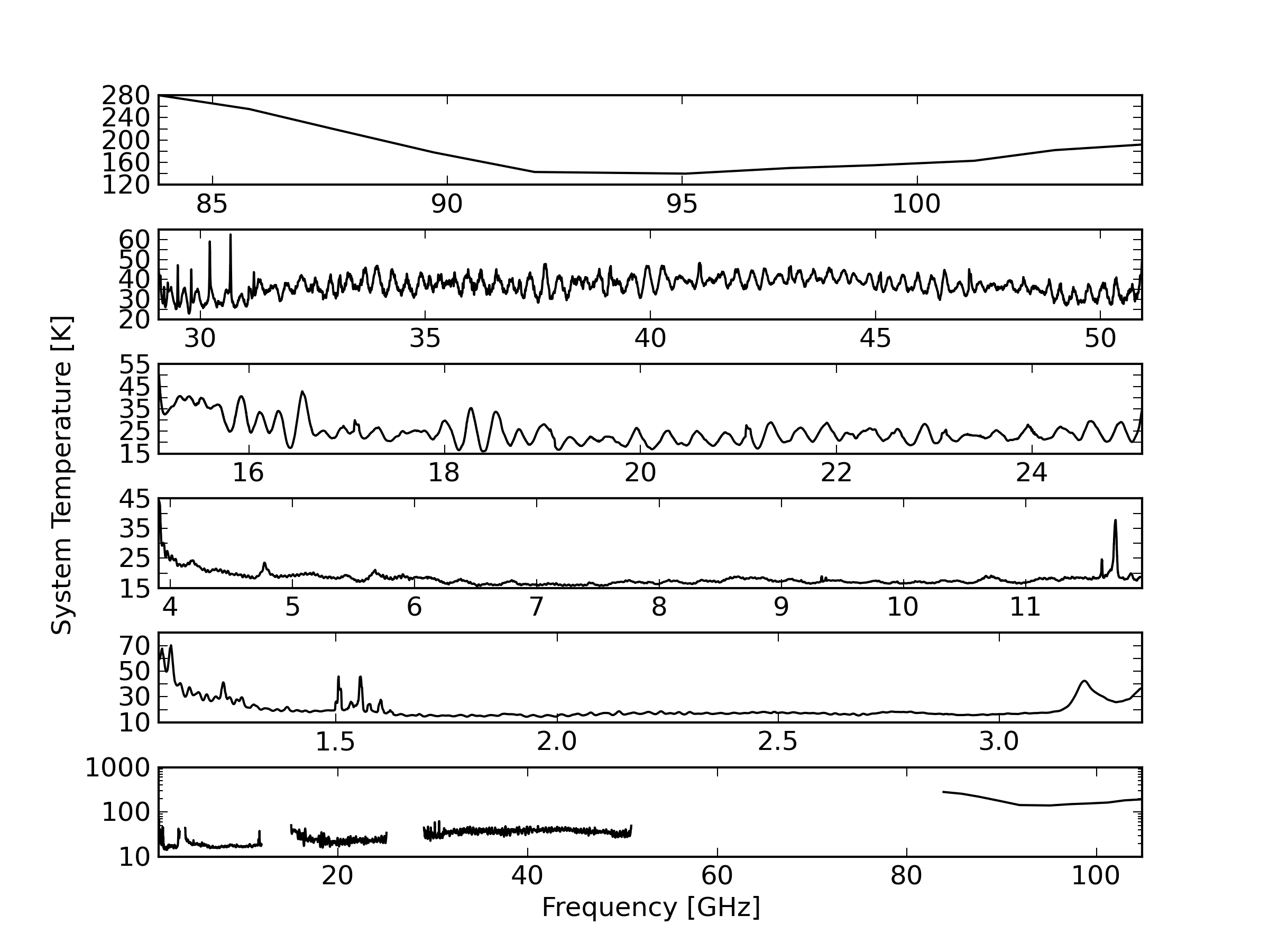
Figure 1.3. Average Compact Array system temperatures for each observing band at high elevation under reasonable observing conditions. These are based on hot-cold load measurements, and include the atmosphere at the time of observation, thus representing the total system temperature. These measurements were made by J. Stevens with the CABB system, except for the 3mm measurements which were made by T. Wong in September 2004.
You can also switch automatically to other wavelengths within tens of seconds (with the exception of the 7mm band as described previously). Similarly the 16cm receiver has a single feedhorn and observations with this package will cover the entire 1.1 - 3.1 GHz range simultaneously. Observations at two simultaneous frequencies are possible in the 4cm, 15mm, 7mm, or the 3mm bands. With CABB, the centre frequencies of the two IFs need to lie within 6 GHz of each other, and even this might be too much separation depending on the exact frequencies chosen. For CABB, the nominal standard frequencies for continuum observations are
2100 MHz in the 16cm band,
5500 MHz and 9000 MHz in the 4cm band,
16700 MHz and 21200 MHz in the 15mm band,
33000 MHz and 35000 MHz in the 7mm LSB band,
43000 MHz and 45000 MHz in the 7mm USB band,
93000 MHz and 95000 MHz in the 3mm band.
These frequency designations follow the ATCA custom of stating the central frequency of the chosen observing frequency range. (For archival data from the pre-CABB era the standard frequencies were
1384 MHz and 2368 MHz in the 20/13cm band,
4800 MHz and 8640 MHz in the 6/3cm band,
18496 MHz and 19520 MHz in the 12mm band,
34496 MHz and 34524 MHz in the 7mm LSB band,
44096 MHz and 44224 MHz in the 7mm USB band,
93504 MHz and 95552 MHz in the 3mm band.
The 15mm recommended CABB central frequencies have recently been changed from 17000 and 19000 GHz, due to the presence of RFI from a geostationary satellite (see Section 1.3.2.3 for details).
Switching between the different frequency bands involves a changing the feed horns. The different feed horns are mounted on a "turret" which rotates the appropriate feed horn to the on-axis position. This is done automatically under computer control and takes about 20 seconds. Turret rotation should be limited to once every 15 minutes unless a compelling scientific case is made for more frequent rotations. The additional overhead in changing to or from 7mm has been described earlier in this document.
Observing-band centre frequencies may be set to the nearest MHz only and no on-line Doppler tracking is done.
Observations of weak H 90α recombination lines may be affected by a trapped mode in the 6/3cm horn at 8857 ± 18 MHz. This trapped mode may enhance the power received this recombination line at their rest-frequency. There are also notches reported in the passband due to trapped modes in the receiver waveguides at 4550 ± 10 MHz, 5328 ± 10 MHz and 8780 ± 10 MHz which may need to be flagged during data reduction.
Both terrestrial and satellite emitters cause radio frequency interference (RFI) to ATCA observations, with the lower frequency bands being more adversely affected than the higher frequency bands. This section describes the RFI that is known in each of the ATCA bands, and also covers interference caused by the Sun.
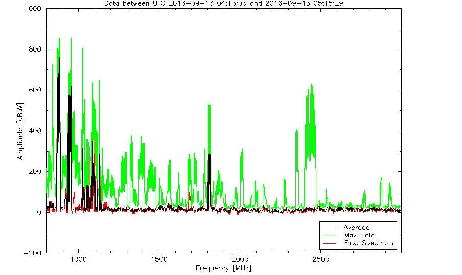
The interference is worse at lower frequencies with the main offenders being microwave links, microwave TV, microwave ovens, navigation satellites and self-generated interference. There can also be significant interference at 1381 MHz from the GPS L3 beacon on occasions. These channels may have to be removed from the data. Figure 1.4 shows what the ATCA sees in its 16cm band (centred at the recommended continuum central frequency of 2100 MHz) when fringe-rotation is disabled (achieved by setting the phase centre to be the South celestial pole). The black, red and blue lines show the log of the amplitude as observed by surveys in 2011, 2015 and 2018 respectively, and from this we can see that the RFI environment does change slightly over time. No self-generated interference is visible in this plot. The Australian Communications and Media Authority (ACMA) band licenses are shown on the plot as coloured frequency regions. The strongest sources of RFI are mobile phone towers, satellites and TV transmitters, all of which are relatively stable in time.
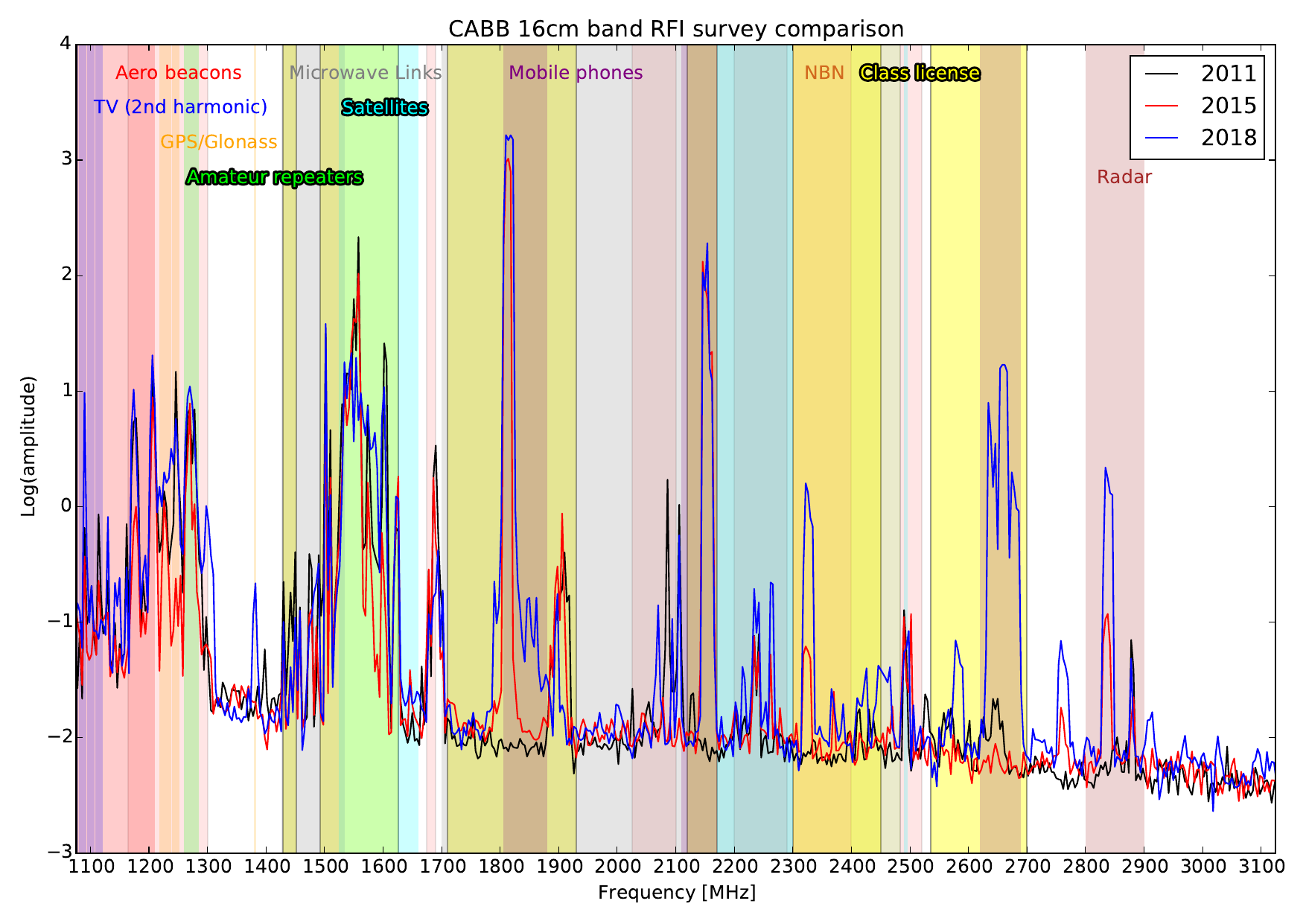
Figure 1.4. The ATCA 16cm RFI environment. Three surveys are shown, one from 2011, one from 2015 and another from 2018. The licenses applicable to each frequency range are shown as coloured regions, labelled with a similar colour at the top of the plot.
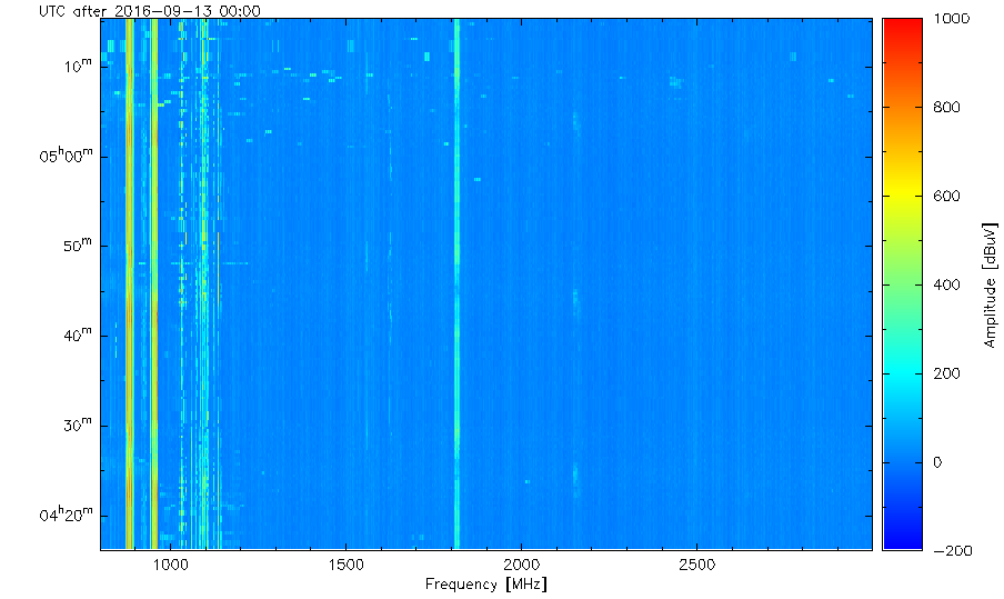
An RFI monitoring antenna sits atop the central control building at the observatory. It monitors the frequency range 700 - 3000 MHz once every 20 seconds, with 2 MHz frequency resolution, and presents its data in near-real time on a web page. Three different plots are presented on the page: a “latest spectra” plot (Figure 1.5), a waterfall plot showing the last hour of data (Figure 1.6), and a plot that may help in determining the direction from which RFI is being observed (Figure 1.7). The latest spectra plot always shows the earliest spectrum obtained by the monitor in the displayed time range, along with a “maximum hold” value for each channel over the last hour and the time-averaged power for each channel. The waterfall plot is useful for seeing emission switch on or off over the last hour. You can also scroll back in time for the past day in half-hour increments for each of the plots.
All data from the RFI monitor is archived. A page showing the RFI waterfalls from ATCA
and Parkes each day from 6am to 8pm (local time) is available at
this link.
If you want to get the output of the monitor for any particular time range since
its installation in November 2014, please contact <Jamie.Stevens@csiro.au>.
In addition to the “normal” RFI in the 16cm band, as shown in Figure 1.4, you may also see something dubbed “mid-week RFI”. This RFI has frequency peaks around 1265 and 1300-1310 MHz, and can have extremely high amplitudes. The RFI monitor can be used to see when mid-week RFI is present, as shown in Figure 1.8. Because of the strength of this RFI, it can often drive the front-end system of the 16cm receivers, or the CABB digitisers, into saturation, or at least produce very large intermodulation products since each tone will act as another LO; if this occurs, the data becomes unusable. We do now sometimes receive advanced warning on when this RFI may be present, and if this will affect observations, the investigators will be notified so they can plan how to deal with it.
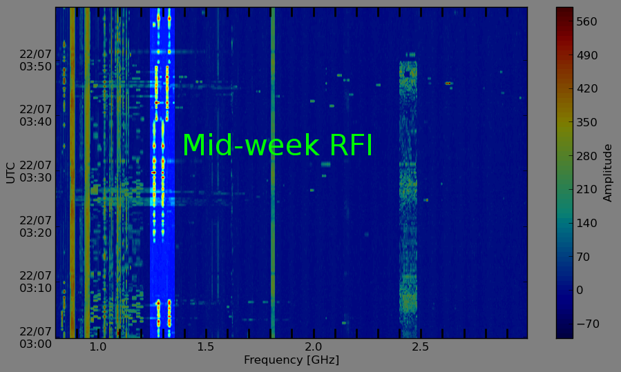
Figure 1.8. A waterfall plot from the RFI monitor, showing what “mid-week RFI” can look like (in the brighter region).
Only the 16cm band is affected by mid-week RFI, so if mid-week RFI is forecast during your observations, you may wish to avoid using the 16cm band during those times, wherever possible. If this is not possible, you may ask for a schedule swap, but this may not always be a possibility. Our observations have also shown that mid-week RFI is present only for a small fraction of the default CABB 10 second cycle time, but is so strong that it ruins the entire integration. You may therefore be able to cope with mid-week RFI by running with a shorter cycle time (say 1 or 2 seconds) and flagging those cycles in which the RFI is present; this will result in a much higher data rate of course, and is only really suitable for continuum experiments that do not need mosaicking.
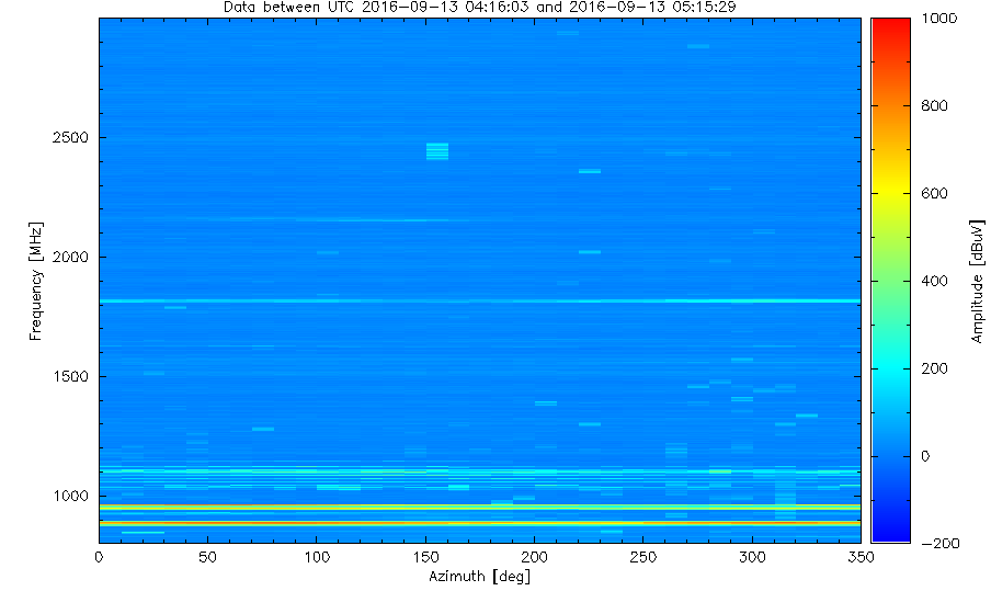
The RFI present in the 4cm band is direction dependent, and can be quite variable over time. Using a similar survey technique to the 16cm band, where the fringe-rotation is disabled, we can determine the static levels of RFI. We also use the antennas to determine how directional the RFI signals are, by doing the survey twice; once while the antennas are pointing at the South Celestial Pole (SCP, Figure 1.9), and again while pointing at the celestial equator (Figure 1.10). We expect that signals coming from satellites will be stronger towards the celestial equator.
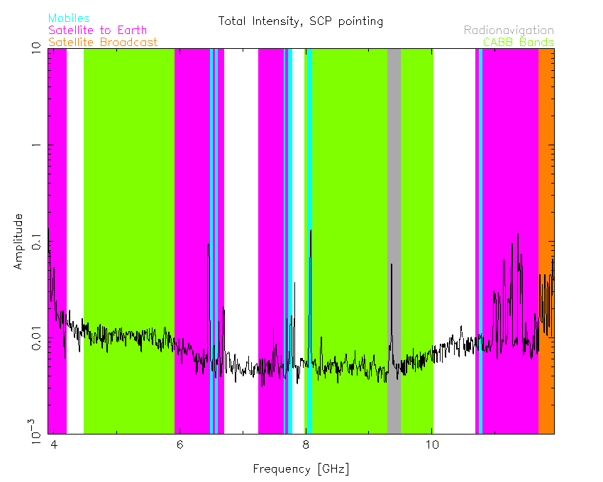
Figure 1.9. The 4cm band, as observed during an RFI survey from 2016-09-07, while the antennas were pointing at the South Celestial Pole (SCP). The colour bands show frequency ranges that represent either the CABB recommended continuum bands, or the ACMA licence applicable.
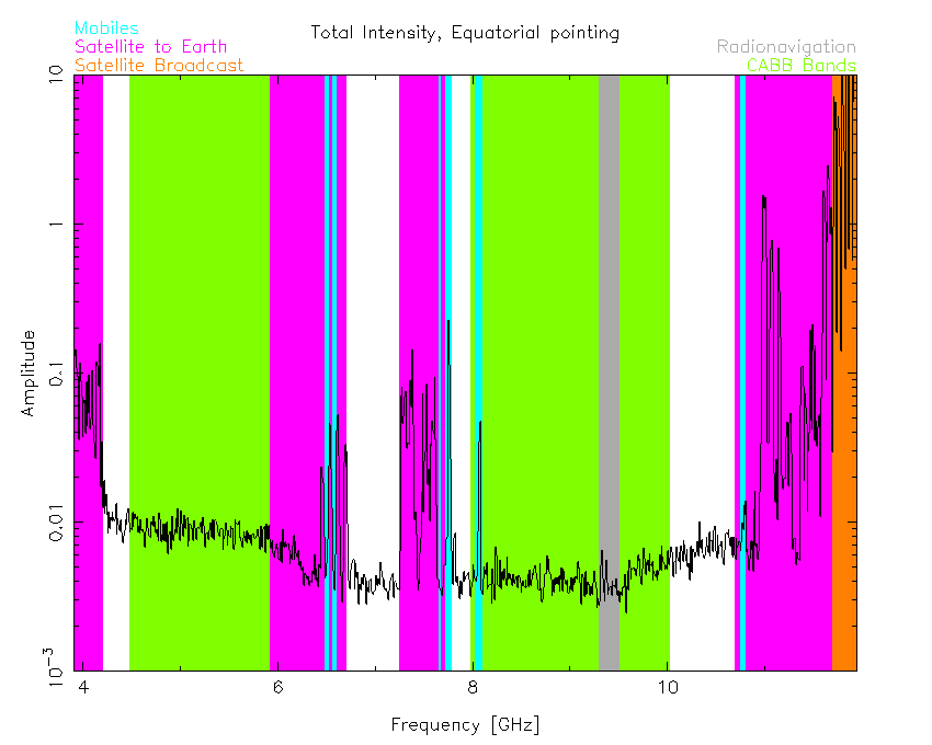
Figure 1.10. The 4cm band, as observed during an RFI survey from 2016-09-07, while the antennas were pointing at the celestial equator at transit. The colour bands show frequency ranges that represent either the CABB recommended continuum bands, or the ACMA licence applicable.
Indeed, we see that in the pink- and orange-highlighted regions of those two figures, the signal intensity is higher while pointing at the equator. That is, in the frequency bands licenced for satellite communications to Earth, the ATCA will see a lot more interfering signal while observing near to the equator. The frequencies of these highlighted regions are given in Table 1.2.
Table 1.2. Frequency ranges of satellite emission bands observed with a 4cm RFI survey. The ranges given are delimited by ACMA allocations, so several entries may be given even if they represent one contiguous frequency range.
| Purpose | Frequencies | |
|---|---|---|
| Low [GHz] | High [GHz] | |
| Communications to Earth | 3.6 | 4.2 |
| 5.925 | 6.7 | |
| 7.2525 | 7.3775 | |
| 7.375 | 7.45 | |
| 7.45 | 7.55 | |
| 7.55 | 7.75 | |
| 10.7 | 11.7 | |
| Broadcast to Earth | 11.7 | 12.2 |
The other frequency ranges shown on Figure 1.9 and Figure 1.10 encompass RFI that is not likely to be from satellites, but as can be seen, the intensity of this RFI is not high and should be easily excisable during data reduction.
There appears to be no significant interference within the 7mm and 3mm bands. An RFI survey in the 15mm band showed that interference from the Australian National Broadband Network (NBN) satellite “Sky Muster” is clearly visible when pointing toward the equator. Similar to the 4cm RFI survey technique, Figure 1.11, Figure 1.12 and Figure 1.13 show that the signal received by the antennas from this satellite (soon to be two satellites) is very dependent on the pointing direction.
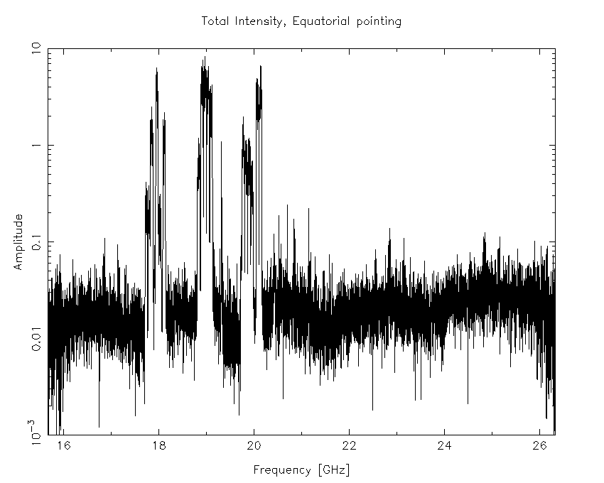
Figure 1.11. The 15mm band, as observed during an RFI survey from 2016-08-01, while the antennas were pointing at the celestial equator at transit.
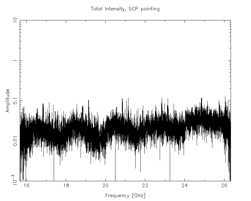
Figure 1.12. The 15mm band, as observed during an RFI survey from 2016-08-01, while the antennas were pointing at the South Celestial Pole (SCP) at transit.
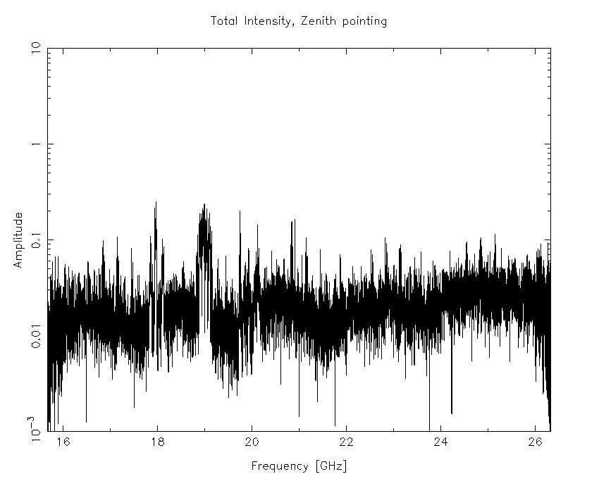
Figure 1.13. The 15mm band, as observed during an RFI survey from 2016-08-01, while the antennas were pointing east at an elevation of 85°.
The “Sky Muster” satellite emits in three broad downlink frequency ranges. These ranges are 17.7 - 18.2 GHz (Figure 1.14), 18.8 - 19.3 GHz (Figure 1.15) and 19.7 - 20.2 GHz (Figure 1.16).
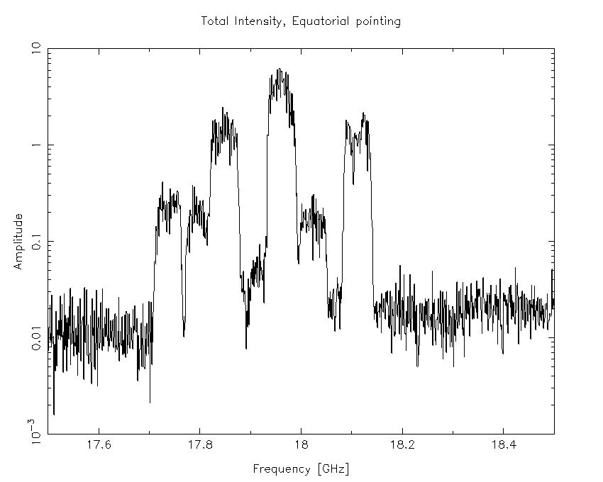
Figure 1.14. A subset of the 15mm band, as observed during an RFI survey from 2016-08-01, while the antennas were pointing at the celestial equator. This frequency subset covers the “Sky Muster” downlink range 17.7 - 18.2 GHz.
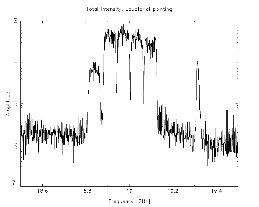
Figure 1.15. A subset of the 15mm band, as observed during an RFI survey from 2016-08-01, while the antennas were pointing at the celestial equator. This frequency subset covers the “Sky Muster” downlink range 18.8 - 19.3 GHz.
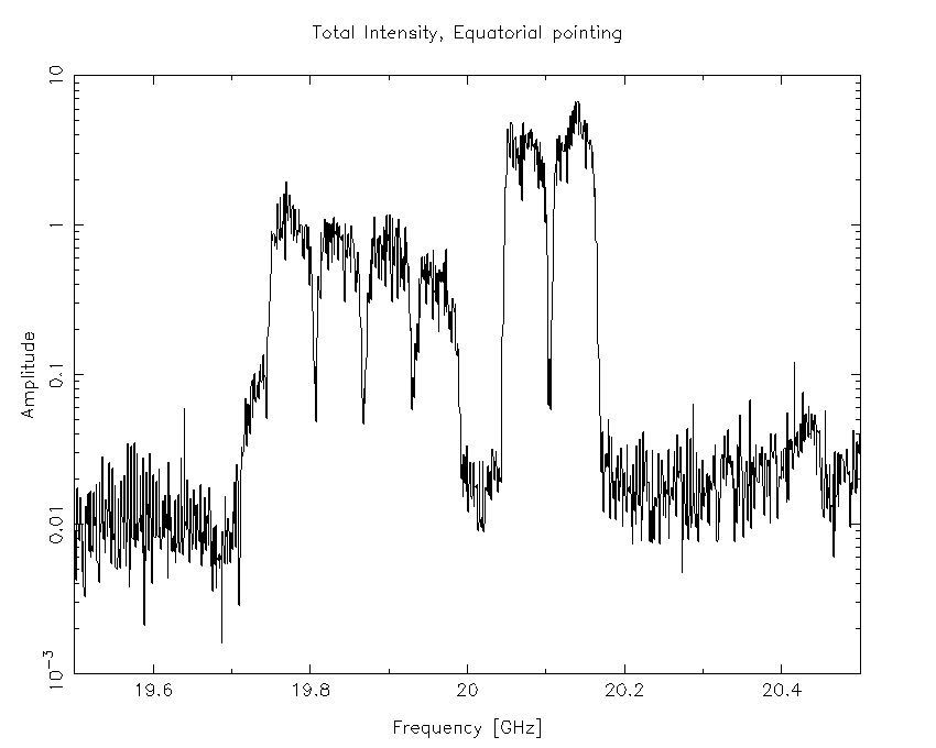
Figure 1.16. A subset of the 15mm band, as observed during an RFI survey from 2016-08-01, while the antennas were pointing at the celestial equator. This frequency subset covers the “Sky Muster” downlink range 19.7 - 20.2 GHz.
This geostationary satellite is at an azimuth of 341.5° and elevation of 53.1°, as seen from the ATCA. This corresponds to a declination of +6° 35′ and hour angle of +1h 14m (west of transit). This position is approximately 18.9° away from pointing position of the antennas during the RFI survey, so the intensity of the interference can be expected to be much higher than shown in Figure 1.11 for pointings closer to the satellite.
The recommended CABB continuum central frequencies for the 15mm band were 17 and 19 GHz, but these may now contain a significant amount of RFI from “Sky Muster”, depending on where your source is. If you are worried about this interference and wish to avoid it, we recommend a new set of continuum central frequencies of 16.7 and 21.2 GHz. These recommended frequency bands are not contiguous, but do avoid all the “Sky Muster” downlink emissions and in fact are slightly more (between 3 and 10%) sensitive than the 17/19 GHz bands in good dry weather where the atmospheric water content is low. If you need to use the 17/19 GHz bands now in order to facilitate comparisons to data obtained in the past, you will likely need to do extensive flagging during data reduction; the reduced bandwidth lost to flagging will also mean that your continuum sensitivity suffers.
To avoid Solar interference, a rule-of-thumb is to observe at a time of year when your source is further than about 40° from the Sun, where possible. It is recommended to specify in your proposal dates that are not suitable for observations if the Sun angle is too small. Low-frequency observations, particularly in spectral-line mode, should be made at greater Solar separations. You are advised to observe at night in cases where good quality 21cm HI data is essential on the shortest (30m) baseline. For spectral-line observations, software exists in Miriad to model and subtract out solar interference. Some information about solar activity can be obtained from the Bureau of Meteorology Space Weather Services.
A synthesis imaging telescope such as the Compact Array provides a great deal of flexibility when deciding how to image an object. In addition to the well-known trade-off between observing time and sensitivity, we have trade-offs with maximum resolution and with the sampling interval in the visibility plane.
The choice of angular resolution is fairly straightforward. Increased angular resolution (resulting from longer baselines) leaves the point-source sensitivity constant, but decreases brightness sensitivity in proportion to the beam area (see Table 1.4).
The choice of (u,v)-plane coverage is more difficult. The amount of independent information needed to specify the image should not exceed the number of independent (u,v)-plane samples. But unfortunately neither of these “independents” is easily defined. At one extreme, consider making a high resolution image of a complex source filling the entire primary beam. In this case full (u,v)-coverage is obtained by using all baselines between 30m and 6000m in increments of 15m. Although this was theoretically possible (it takes 25 separate array configurations), it was never attempted and, since the decommissioning of the second 6km station, is no longer actually possible!
If on the other hand the image is smaller than the primary beam then the Nyquist sampling interval is larger and the number of (u,v)-samples required is reduced. The observing time can then be reduced either by decreasing the number of configurations or the amount of hour angle coverage, depending on the array configuration. For east-west arrays, reducing the total number of configurations is the more practical option. If the source is large but partly empty it can be considered to have a size corresponding to its area.
For ordinary observations Table 1.4 gives the maximum sizes of structures that can be reliably imaged for typical sets of observing configurations. This is only a rough guide since the actual coverage needed depends on details of the 2-dimensional brightness distribution, on the actual distribution of baselines, and on the type of deconvolution. Additionally, other techniques such as mosaicking and multi-frequency synthesis, can be extremely effective at improving (u,v)-coverage.
A further consideration is the minimum spacing available. This is never less than 30 m and for a given configuration can be much larger. This acts as a high-pass filter removing all Fourier components less than the minimum spacing. If this is a serious problem, short baseline information (e.g., from a single dish) can be added separately during processing.
Antenna 6 sits permanently on station W392. Maximum baselines to this antenna (the last 5 columns) are shown for all configurations in Appendix H, but form part of a designed array only for configurations 6.0A to 6.0D. The antennas can be moved to, and set up on, a limited number of fixed stations. Because of this and other physical restraints, the shortest spacing available is 30 m, the longest is 6 km, and the minimum grating increment is 15 m. From 2006 October, the standard set of configurations has been:
1 hybrid configuration with a maximum baseline length in the North-South direction of 75 m (H75)
1 hybrid configuration with a maximum baseline length in the North-South direction of 168 m (H168)
1 hybrid configuration with a maximum baseline length in the North-South direction of 214 m (H214)
2 east-west configurations with a maximum baseline of about 375 m
4 east-west configurations with a maximum baseline of about 750 m
4 east-west configurations with a maximum baseline of about 1500 m
4 east-west configurations with a maximum baseline of about 6000 m.
Snapshot observations using the Northern spur in hybrid configurations will generate a two-dimensional sampling of the (u,v)-plane. The Northern spur was installed so that good coverage of the (u,v)-plane was achievable for observations which are limited to hour-angles near transit. Observations at mm wavelengths should be limited to higher elevations to avoid large atmospheric opacities. Hybrid arrays are also useful for observations of northern sources which are similarly restricted in hour-angle range.
The 6 km antenna may also be added to any of the shorter configurations, but in these cases the distribution of array spacings is bi-modal.
The predetermined set of configurations offered for forthcoming observing terms will assist in planning multi-configuration proposals. Details of previous configurations and those being offered in coming semesters can be found on our website, or see Table 1.3.
Note that proposals requiring two or more configurations will usually be allotted two or more widely separated times; therefore, expect to make two or more observing visits, or conduct the second observation using remote observing. If you are not allotted all the configurations requested, you should re-apply in the next term, as the proposal will not be automatically reconsidered.
The overall philosophy is that, in each semester, there will be a 6km, 1.5km, and 750m configuration, and for these baselines, the full set of 4 configurations will generally be covered in three semesters. Each semester will also contain at least one 375m configuration. Analysis of user preferences for the past few years show some configurations to be more generally useful (e.g., providing better single-configuration (u,v)-coverage), and it is desirable to offer these more frequently. Millimetre observing conditions are optimal in the (southern hemisphere) winter, so arrays of 214m or smaller will be offered mainly in the April semester.
Table 1.3. Array configurations that will be offered in future semesters.
| Array | Semester | |||||
|---|---|---|---|---|---|---|
| 2021OCTS | 2022APRS | 2022OCTS | 2023APRS | 2023OCTS | 2024APRS | |
| 6A | • | • | • | • | • | • |
| 6B | • | • | ||||
| 6C | • | • | ||||
| 6D | • | • | ||||
| 1.5A | • | • | ||||
| 1.5B | • | • | ||||
| 1.5C | • | • | ||||
| 1.5D | • | • | ||||
| 750A | • | • | ||||
| 750B | • | • | ||||
| 750C | • | • | ||||
| 750D | • | • | ||||
| EW367 | • | • | • | |||
| EW352 | • | • | • | • | • | • |
| H214 | • | • | • | • | ||
| H168 | • | • | • | • | • | |
| H75 | • | • | • | |||
Besides the predetermined configurations, you can request any standard or non-standard configuration in any term. When writing your application, your scientific justification should include a convincing argument of why you need to use a special array configuration, rather than one of those offered for the term. If you need such a “wildcard” request for a significant amount of observing time (e.g., more than 5 x 12h), you can enhance the probability of it being scheduled if you contact ATNF well in advance of the deadline (preferably even before the call for proposals announcement). The wildcard can then be advertised as a potential additional configuration for the term, which may then lead to other proposers requesting it, and making its scheduling viable.
For those who wish to improve their (u,v)-coverage by re-observing on different days with different antenna configurations, specific sets of configurations combines well, e.g., 6A, 6C, 1.5B and 1.5D — for more details see Appendix H.
An interactive tool, the Friendly Virtual Radio Interferometer (VRI), is available to assist users in exploring the (u,v)-coverage of standard (and non-standard) configurations.
It is strongly recommended that the proposer gives a clear indication of the maximum extent of their sources. You should also specify the maximum and minimum baselines, and the number of configurations (days) needed.
The CABB now provides a variety of frequency resolutions. The available resolution options are more commonly denoted by the CABB configuration that is used to provide them. Two correlator configurations are available:
- Currently available modes
CFB 1M-0.5k: 2048 channels per 2048 MHz continuum IF (1 MHz coarse resolution), and 2048 channels per 1 MHz zoom band (0.5 kHz fine resolution).
CFB 64M-32k: 32 channels per 2048 MHz continuum IF (64 MHz coarse resolution), and 2048 channels per 64 MHz zoom band (32 kHz fine resolution).
There is also a “hybrid" mode available which provides one continuum 2048 × 1 MHz IF (with no zoom bands), and a second continuum 32 × 64 MHz IF (with up to sixteen 64 MHz zoom bands).
It should be noted that the correlator routinely computes double the number of channels as is recorded. This second set of channels is offset from the available set by half the channel width, and are there to provide flexibility in choosing the zoom band frequency, as well as to ensure that it will always be possible to avoid observing a spectral line at the edge of a channel. It is also possible to combine a number of overlapping zoom bands that are separated by half a continuum channel into a seamless single zoom band.
The next two sections describe some necessary considerations for both centimetre and millimetre observations at the ATCA. This section on centimetre observations is also relevant for millimetre observers and should be read by everyone planning to propose for the ATCA. The millimetre section describes some additional requirements specific to millimetre observations.
Table 1.4. Continuum brightness temperature sensitivity (12 hr integration) for bandwidth specified in Table 1.1, for various arrays.
| Band | Array | |||||
|---|---|---|---|---|---|---|
| 6km | 1.5km | 750m | EW352 | H214 | H75 | |
| 16cm | 0.02 K | 2.1 mK | 0.53 mK | 0.1 mK | 0.1 mK | 0.02 mK |
| 4cm | 0.01 K | 1.6 mK | 0.4 mK | 0.07 mK | 0.11 mK | 0.01 mK |
| 15mm | 0.02 K | 2.6 mK | 0.65 mK | 0.12 mK | 0.18 mK | 0.02 mK |
| 7mm | 0.03 K | 4.8 mK | 1.2 mK | 0.22 mK | 0.33 mK | 0.04 mK |
| 3mm | — | — | — | 1.4 mK | 2.1 mK | 0.24 mK |
It is crucial to obtain good calibration data during your observations, and you must consider how much of an overhead calibration will represent before you propose an experiment. A detailed description of the calibration required is given in Section 2.2.
The amount of calibration required will also depend on when the experiment is scheduled. Observations requiring maximum phase stability (e.g., at wavelengths less than 6cm) should be made in winter, or at night.
The general expressions for the flux and brightness sensitivities are given in the document AT/01.17/025, and these general expressions have been used in Table 1.1. The observer has control of the integration time (), bandwidth (B), observing wavelength (), number of baselines (N) and synthesized beam size () only, and with these variables and the system sensitivity (), the expressions reduce approximately to:
and
where is in Jy, in min, B in MHz, in cm, and is in arcsec. For the full 6 km array, N=15. There is a convenient ATCA sensitivity calculator which takes into account system temperature, observing frequency, array, correlator configuration and (u,v)-weighting. (A pre-CABB version of the calculator is also available on the ATCA web page for use when considering the utility of archival ATCA data.)
Technical details of the ATCA mm systems are presented in MMICS for the AT mm-wave receiver system by Gough et al. (Proc. 12th European Gallium Arsenide and other Compound Semiconductors Application Symposium, 2004, pp.359-362) and Cryogenically Cooled mm-wave Front Ends for the Australia Telescope by Moorey et al. (Proc. European Microwave Conference, 2008, pp.155-158). This section builds on many of the concepts described in the previous section on centimetre wavelength observations, which should be read before reading this section.
All six antennas of the Compact Array are equipped with 15mm receivers covering the frequency range 16–25 GHz. The 15mm system shares a common dewar with the 7mm and 3mm receivers, and the separate feed horns at the top of the dewar are moved to the Cassegrain focus of the Compact Array antennas using the rotator positioning system. Because the 15, 7 and 3 mm receivers have separate feed horns, observations cannot be simultaneous between the 15, 7 and 3 mm bands.
The ATCA can observe within the frequency range 30–50GHz. Feeds and receivers were installed into the existing mm-wave receiver packages on all 6 antennas in 2007, with the 7mm upgrade jointly funded by the ATNF and NASA's Deep Space Network to enable the ATCA to participate in occasional spacecraft tracking.
The wide 7mm band presents difficulties in signal down-conversion, as the aliased signal from the first down conversion stage can also be within the 7mm band. Although image rejection filters are used, variations in receiver gain across the band, combined with the frequency-dependent performance of the filters themselves, can result in appreciable signal levels being added to the observing band. Generally, this aliased signal does not cross-correlate and is present as a contribution to the noise level. However, in some circumstances, notably as the delay rate drops to zero (e.g., around source transit on north-south baselines), the aliased component can cross-correlate and be visible as “beating" on some baselines. This data must be flagged during the data processing.
The inner five ATCA telescopes (i.e., excluding CA06) are outfitted with a 3mm receiver and can observe in the range 83 to 105 GHz. A noise diode has been added to the 3mm system on CA02 (only) to aid with 3mm polarisation calibration. Aliasing effects similar to those described at 7mm can also arise in the 3mm band.
A limited form of flexible scheduling is operational for observations at millimetre wavelengths. Consult the document Flexible Scheduling at ATCA for details.
A quickstart guide for 3mm observing is also available.
Observations in the mm band are run from a schedule file in the same way as cm-band observations. However, due to the effects of atmosphere stability, mm observations require bandpass and phase-calibration checks at a much more frequent rate.
Note that as ATCA does not Doppler track, it is important to have a good estimation of the magnitude of the Doppler shift for the line of interest. This is particularly so for the higher frequencies available to the 3mm system. The sky frequency can be calculated using an online calculator.
A simple phase reference observation takes about an hour to run, including calibration. The following procedure is typical:
Pointing calibration → Paddle calibration (3mm only) → Bandpass/Phase calibrator → Target source → Paddle calibration (3mm only) → Bandpass/Phase calibration → Target observation.
The CABB web scheduler can be used to construct the observing schedule.
Elevation angles close to the array horizon should be avoided because of the increased opacity and poorer atmospheric stability. Therefore, observations of objects with a declination further north of -50° are best made using hybrid configurations (i.e., one using the N-S spur) in order to achieve sufficient (u,v)-coverage.
Observations using very compact telescope configurations should be made with caution, as telescope shadowing can be a significant problem, especially for sources at declinations which do not achieve elevations high above the horizon. See Section H.2 for details.
You may not wish to make detailed high resolution images but instead, for example, survey a large number of compact or simple sources. Under these circumstances, if the sources are strong enough, short observations will suffice (Table 1.5). In scheduling these, slew time becomes an important consideration; these may be calculated (see Section 1.7.3), or with the use of the CABB scheduler. A single short observation in an E-W array will give a 1-dimensional (u,v)-coverage; two or more short observations will give some 2-dimensional information. In such short observations consequent higher sidelobe levels will exacerbate problems caused by confusing sources in the primary beam. Because the Compact Array has poor (u,v)-coverage, in contrast to its good sensitivity, this confusion makes it difficult to reach the receiver noise limit when observing weak sources or searching for detections, particularly at lower frequencies. Current experience suggests that at 6cm at least 8 short observations well distributed in hour angle are needed to reduce confusion to the noise level. At 16cm, short observations are unlikely to ever reach the noise limit.
Two orthogonal linear polarisations are measured simultaneously. The position angle of the polarisation splitter is stationary with respect to the alt-az–mounted antennas and so rotates on the sky. A suite of tasks in Miriad is available for polarimetric calibration of Compact Array data. No specific calibrators, other than the usual flux and gain calibrators, are needed for polarisation calibration. An observation of B1934-638 is essential when only making short observations. Small drifts with time can be corrected for using the on-line measurements of the XY phase differences to an accuracy of 0.5 degrees at all bands. Best polarimetric calibration results when the gain calibrator is observed at a good sampling of different parallactic angles.
Miriad is routinely used to calibrate data in all bands, with consistent results being achieved over several months in the cm bands. The on-axis instrumental polarisation is typically below 2-3%. After calibrating for instrumental polarisation, we are currently able to reduce on-axis instrumental effects to 0.1%, and better with some care.
The off-axis polarisation increases roughly as the square of the distance from the pointing centre at least up to the half-power point. At 16 and 4cm, the instrumental polarisation is about 3% of the apparent total intensity at the half power point, respectively. This error is almost purely linearly polarised (there is no circularly polarised component). Because the ATCA antennas have an alt-az mount, the off-axis response varies with parallactic angle, and will be smeared out by a factor of a few by a long synthesis. This smearing is a function of declination. The Miriad task offpol can be used to simulate off-axis polarimetric response of a long synthesis observation. Mosaicking smears out the off-axis response still further, by as much as an order of magnitude.
At 16cm, instrumental polarisation is largely independent of frequency. The leakages are now flat to better than 2% across the entire usable band. More detail on the polarisation properties of the ATCA 16cm receivers can be found in the receiver commissioning report.
Objects which are of similar size or larger than the primary beam will need to be mosaicked. In such cases, the recommended spacing of pointing centres is half of the primary beamwidth. The Compact Array antennas and control system allow for rapid switching between pointing centres — as frequently as once per integration cycle. This enables a source to be rapidly mosaicked without necessarily losing (u,v)-coverage. The antenna acceleration limit is 800 deg/min/min, and the slew limit is 38 deg/min in azimuth and 19 deg/min in elevation. Mosaicking mode may also be useful for observing large numbers of nearby sources, as the observing overheads are reduced.
There is also a facility for “on-the-fly" mosaicking, whereby the antennas are continuously driven. This type of mosaicking may be especially useful for large-area mosaics at low frequencies, where the drive times between mosaic pointings are significant.
Section 2.3.4 explains how to set up mosaic files. The Miriad User Guide describes how to reduce a mosaic data set.
As (u,v)-distance is proportional to frequency as well as baseline length, different (u,v)-spacings can be obtained not only by varying the antenna configuration, but also by varying the frequency.
Additional (u,v)-coverage can be obtained in the mm bands by observing at multiple frequencies. Observing at two frequencies has the added advantage of increasing sensitivity, as they can be observed simultaneously. Observing more than two frequencies requires time sharing. While this will not improve the sensitivity further, it can significantly improve the (u,v)-coverage. However, there is a trade off between gaps in the tangential and radial directions in the (u,v)-plane. Typically two or three pairs of frequencies, observing each setting for 10 minutes, is a good compromise.
When you use both bandwidth synthesis and two or three configurations, and require (u,v)-coverage to 6km, the best choice of configurations is not two or three 6km arrays, but a combination of 6km with 1.5km and 750m arrays (all arrays using the 6km antenna). The flux density of most sources will often vary significantly between different frequencies and, furthermore, this variation itself (i.e., the spectral index) will vary across the source. This complicates the task of combining data from the different frequencies when you want high-dynamic-range images. However software is available in Miriad to account for the spectral variations in the imaging, deconvolution and self-calibration steps. These algorithms solve for, or use, both a basic flux-density image and a spectral-index image. For typical spectral indices, they are appropriate for frequency ratios less than about 1.25.
After each antenna reconfiguration a pointing solution is determined. Generally, rms errors of around 5 arcsec are achieved at this time. These solutions degrade with thermal (and other) effects. By the time observations are undertaken, rms errors of about 10 arcsec (or more) are likely. There is a significant offset (of up to 30 arcsecs) between the mm and the cm receivers.
A reference pointing mode is available which is recommended for mm observations. In this mode, a 1 Jy calibrator, about 5° to 10° away from the target will hold the pointing to 10 arcsec rms. A bright (say 5 Jy) calibrator at 2° to 3° from the target will reduce the errors to about 5 arcsec rms. A reference pointing scan generally takes 2-3 minutes to complete. See the Reference Pointing Guide for details.
In pulsar binning mode, the correlator cycle time (normally 10 seconds) is divided into an integer number of pulsar periods. Each pulsar period is further divided into N equal time intervals called bins. The integration in the correlator is done separately for each bin, such that at the end of the cycle, N quantities are produced, each of which represents the integrated value at a particular pulsar phase. The minimum time bin is around 110 micro-seconds, allowing, for example, 32 phase bins for a 3.5 milli-second pulsar. The correlator will also record both the full 2 GHz continuum bands in addition to the pulsar binning data, analagous to how the zoom modes are recorded. However, the binned data has lower frequency resolution (by a factor of 4) than the unbinned continuum data.
For high time resolution observations, a time resolution of order 10 milliseconds is possible, though with a reduced number of channels across each 2 GHz band (achieved by averaging over 1 MHz channels).
The Compact Array can track sources with non-sidereal rates, such as planets or comets. In this case delay tracking is adjusted continuously to account for source proper motion. The antenna pointing also correctly tracks non-sidereally.
JPL ephemerides of the planets are built into the observing program, and a simple mechanism exists to import current JPL ephemerides of other solar system objects (e.g. new comets).
A tied array capability is available. It provides tying of the array at one or two frequencies and, for CABB, at a bandwidth of 64 MHz.
The tied array adder is controlled via a process called catie which
runs within cacor. This allows the choice of which antennas are
included and whether the adder produces linear or circular
polarisation outputs. The array is phased up in the usual way, and an
option to allow the insertion of a 90° phase offset
between the A and B linear polarisations at each antenna – thereby
forming circular polarisation at the tied-array output – is available.
The tied-array adder is fed into the LBA (Long Baseline Array) DAS which provides outputs for the VLBI disk-based recorders at bandwidths between 62.5 kHz and 64 MHz. Simultaneous Compact Array and tied array operation is possible, although currently this is limited to 64 MHz in both IFs, or 64 MHz in one IF and the full 2 GHz (which is not formed into a tied array) in the other.
The presence of field sources in the primary antenna beam can limit continuum image quality. These sources produce unwanted sidelobes in the images and can lead to dynamic range and aliasing problems. The brightest source expected on average in the half-power primary antenna beam (away from the Galactic plane) is listed in Table 1.1. Note that confusion becomes much worse as you go to lower frequencies, and that this can be particularly serious for snapshot observations (See Section 1.7.1). The SUMSS catalogue and database, and the Molonglo Galactic Plane Survey (MGPS-2) catalogue and database are useful references to search for potential confusing sources in the 16cm band, where the effects of confusion are greatest.
At short wavelengths and/or long baselines, atmospheric refraction can cause serious phase errors. The problem becomes progressively less serious at longer wavelengths and shorter baselines. Atmospheric conditions are most favourable during winter and at night. A seeing monitor at Narrabri continuously monitors the phase stability at a frequency of 21 GHz and over a baseline of 200 m. See The ATCA Seeing Monitor for details (though note this paper describes the initial system; in 2008 a new satellite beacon was adopted, resulting in a change in the frequency from 30GHz to 21GHz, and the design was changed again in 2019 when the satellite we were using became non-geosynchronous).
High winds, storms and extreme heat can damage the antennas. See Section 3.5.1 to Section 3.5.3 for further details on automated stowing procedures.
As with other synthesis instruments, system errors such as DC offsets and sampler harmonics can lead to artefacts at the centre of the field. These artefacts have not yet been observed to affect the data from the CABB correlator, but if such an error would severely degrade your science goals (e.g. in a detection experiment), it is preferable to displace the source positions a few (synthesized) beamwidths from the field centre.
The Compact Array operates under a semester system with two application deadlines each year: around June 15 for observations from October 1 to March 31; and around December 15 for observations from April 1 to September 30. During each semester array maintenance, upgrades and array reconfigurations (moving the antennas to different stations) are scheduled in addition to astronomical observations. Target of Opportunity (ToO) requests for observations of extremely important transient or non-predicted events can be made at any time. To learn how to apply for ToO observing time, visit our webpage.
Based on previous experience, observing at 3mm usually ends by October 15, restarting in late April. Detection experiments at 7mm and 15mm usually end by October 31, restarting in early March. Observations of bright compact sources, for which self-calibration is possible, may be made throughout the year. Observations at times other than those indicated above require an explicit justification in the proposal.
Check our web page for information about the current status of the ATNF facilities. Before submitting proposals to observe particular objects, you should check that the observation you are proposing has not already been made. Previous Compact Array proposals and observations can be found in the ATOA (Australia Telescope Online Archive). After the proprietary period has expired, the data files from previous observations may be downloaded from ATOA.
All ATNF Telescope Applications must be submitted using OPAL.
After the Time Assignment Committee (TAC) has met, you will be notified when the TAC grades and feedback on your proposal are available. These are available to all members of the proposal team through OPAL. All proposers are notified when the schedule for the next semester is released, and these schedules will appear on the web.
Generally, at least one member of the observing team must be present at the SOC to do the observations. The visiting observer should be well-versed with the needs of their observing program before arriving, particularly if they did not write the observing proposal or schedule files. If they need assistance from the DA to prepare their schedules, they should arrive well before the start of their observations; at least two weekdays.
Occupational Health and Safety regulations require that observers are not to observe for more than 16 hours, so for long observations you will need more than one observer.
Plan your trip to the SOC with the help of the ATNF Visitor's Information. You will need to book transport, accommodation and computer resources in Marsfield before arrival.
Note that multi-configuration observations are likely to occur weeks or even months apart, so you may need to plan either one long visit or several short trips. Overseas observers will require a valid visa and passport for entry into Australia.
The Compact Array is controlled from user generated schedule files. Schedule files are prepared with the CABB web scheduler.
Schedules contain source names, positions, frequencies, bandwidths, and any other information that caobs needs for observations.
A useful tool to determine the altitude, azimuth, and rising and setting times of astronomical objects, which may help with preparation of your schedule files, is the Interactive Observability Chart Plotter.
A Duty Astronomer will be present at the SOC to help local observers get their observations started, and to help with any problems that arise during the observations. Our web site has the list of duty astronomers for the upcoming semester, as well as for previous semesters. The Duty Astronomer has no obligation to participate in the observing. For remote observers, the DA is primarily there to help as problems arise, as qualified remote observers should not need assistance to start their observations.
The ATCA is responsive to requests for observations of targets of opportunity. There are two paths to such observations: through a NAPA (non-apriori assignable) project, or through a ToO (target of opportunity) request.
A NAPA project is one whose science goals have been set down in a proposal that the TAC has evaluated in the normal way. Such projects can be triggered any time during the semester, whenever the investigator wants to proceed. The project will have requested a specific amount of time for the semester, and this is the amount of time that can be displaced from scheduled observations to accommodate the NAPA project. However, if the NAPA requires further time, it can be granted using unallocated time.
A ToO request can also be made at any time during the semester. Unlike NAPA projects though, a ToO will not generally be allowed to over-ride a scheduled observation.
The first step to either trigger a NAPA project, or request a
ToO observation, is to email either the alerts exploder
(<alert@atnf.csiro.au>) or the scheduler directly
(<Jamie.Stevens@csiro.au>); the former is preferable since there is a greater
chance of someone seeing the request quickly.
For a NAPA trigger, you should include in your email the NAPA's project code, and some details about the source(s) you are triggering on, including at least right ascensions and declinations. For a ToO request, you should also include a short scientific justification for why you want to observe.
If you are requesting a slot of Director's discretionary time (also known as green time), then you should also put in a request via the Portal's booking system. If you require an over-ride of scheduled time (only available for NAPA projects), then please state your preferred observation time in your email.
Since the beginning of the 2017OCT semester, it has been possible for almost any NAPA project to over-ride almost any scheduled project. Any exceptions to this will be made clear in the release notes for the semester, and will be communicated privately to the investigators of NAPA projects who cannot avail themselves of over-rides.
The observatory will try to make contact with NAPA requesters as quickly as possible after a trigger has been issued, but sometimes it might not be possible to reach observatory staff (eg. overnight, at weekends, etc.). If the investigators think it necessary, NAPA projects may over-ride scheduled observations without further consultation with observatory staff. We recommend that in such a case, the investigator wishing to over-ride communicate with the current observer in charge to effect the change to the NAPA. It should be noted though that if the NAPA project has already used up the time that it requested for the semester, it is no longer entitled to over-ride scheduled time and must use Director's time instead.
In the case that a NAPA investigator wants to start observing, and the telescope is idle, the current time is unallocated, and there is no observer in charge, they may proceed without any further consultation. This is true for any NAPA project, even those which may not have achieved the grade required to over-ride scheduled time. The investigator must though notify any observers who may want to start their scheduled observations. Even if the time is unallocated, the telescope is idle, and there is no observer in charge, a ToO observation should not assume control of the telescope without permission from observatory staff, since it may be that their science request conflicts with another scheduled project.
For NAPA projects which require very prompt response to a trigger, we recommend the use of the rapid response mode (Section 2.5). Use of this mode is limited in the same way as for a normal NAPA, but an email request does not need to be sent prior to the trigger, and the observing system will manage the transition to the NAPA observations automatically. The investigators of each project that is over-ridden by a rapid response trigger will be notified by email of the displacement, at the time of the trigger.
Otherwise, observatory staff will try to find a time that maximises the science output of the NAPA or ToO request, and minimises the disruption to scheduled time. In any event, all affected investigators will be notified by email as soon as possible after the decision is made.
If multiple requests are received to look at the same target, then staff will need to decide how to allocate the time. In general, NAPA projects will be prioritised over ToO requests, because the TAC has already evaluated the science cases for the NAPAs. This will hold even if the NAPA project has exhausted its time allocation for the semester. If multiple NAPA requests are made for the same target, then both the TAC ranking score and the order in which the requests were received will be considered.
It is possible for one NAPA to be over-ridden by another NAPA, if the observatory staff think it appropriate to do so. In such a case, it would be inappropriate for a NAPA investigator to take control of the telescope without first consulting with observatory staff.
Rapid response observations are a special case: the automatic system does not need staff interaction to work, and so if a rapid response request arrives while another NAPA project is being observed, the rapid response over-ride will take priority. Once a rapid response over-ride is being observed, it must be allowed to run for its allocated duration, and the automatic system will reissue the over-ride should the observation be interrupted. Observatory staff do though have the power to stop a rapid response over-ride observation if necessary.
| Revision History | ||
|---|---|---|
| Revision 1.6 | 2021 October 15 | jbs |
| Improved some sloppy language. Fixed links where necessary. Updated recommended frequency table. Fixed incorrect channel numbers for 64 MHz mode. Fixed 4cm focus statement. Removed advice to observe solar system objects with UTC schedules. Stop linking to obsolete remote observing pages and the current issues page. Removed references to friends. Updated information about how rapid response mode works now. Changed the portal booking picture and updated to reflect how it now works. | ||
| Revision 1.5 | 2017 June 1 | jbs |
| Added information about how to use the rapid response mode | ||
| Revision 1.4 | 2016 May 9 | jbs |
| Updated information about the new high-frequency 1934-638 flux density model | ||
| Revision 1.3 | 2015 Oct 21 | jbs |
| Updated information about remote observing procedures | ||
| Revision 1.2 | 2014 Oct 15 | jbs |
| Fix a couple of typos regarding 1934-638 flux density models | ||
| Revision 1.1 | 2014 May 28 | jbs |
| Rewrite chapter in FAQ format | ||
| Revision 1.0 | 2014 Mar 20 | jbs |
| Initial Docbook revision | ||
This chapter deals with how to prepare for observations on the ATCA after having been granted observing time. It is presented as an FAQ, so that new observers can get all the information they need, and experienced observers can quickly find the information they need.
Broadly speaking you will need to address at least the following considerations when planning an observation with the ATCA:
How much integration time is required on source to reach the necessary sensitivity?
What calibration is required to ensure the observations succeed, and how much observing time will it require?
How can observational overheads be minimised?
How will weather and RFI affect the observations?
After reading this chapter you should be able to optimally plan an observation, and know how to make the schedule that carries it out.
The ATCA antennas have a hard elevation limit of 12°, and for observations in the millimetre bands it is recommended that you stay above an elevation of 30° in order to avoid the thickest parts of the atmosphere.
A quick estimate of how long a particular source will be observable on a single day with the ATCA can be made using Table 2.1. It shows, for a source at a particular declination, the LST range before/past transit it is above elevations of 12° and 30°.
Example: The source 0823-500 (coordinates RA=08:25:26.869, Dec=-50:10:38.4) will rise above the 12° elevation limit at an LST of 01:05 (take 07:20 from 08:25), and it will fall below 30° at an LST of 13:42 (add 05:17 to 08:25). It will be above the 12° elevation limit for approximately 14 h 40 m each day.
Table 2.1. For sources at particular declinations, this table displays the amount of time the source would take to get from rise to transit, or from transit to set at the ATCA. The LST ranges are shown for both the hard 12° and the recommended millimetre 30° elevation limits.
| Declination | LST range | |
|---|---|---|
| 12° | 30° | |
| -80° | always above horizon | 06:09 |
| -70° | 10:35 | 05:47 |
| -60° | 08:14 | 05:32 |
| -50° | 07:20 | 05:17 |
| -40° | 06:44 | 05:02 |
| -30° | 06:17 | 04:46 |
| -20° | 05:53 | 04:28 |
| -10° | 05:31 | 04:07 |
| +0° | 05:07 | 03:42 |
| +10° | 04:42 | 03:09 |
| +20° | 04:12 | 02:20 |
| +30° | 03:32 | 00:21 |
| +40° | 02:31 | never above horizon |
To calculate precisely how long your source is observable each day with the ATCA you can use the Interactive Observability Chart Plotter.
CABB makes available two 2048 MHz wide bands, and the centre frequency of one IF must be within 6 GHz of the centre frequency of the other. Generally speaking however, the closer the two centre frequencies are to each other, the more sensitive the observations will be.
This is due to the design of the CABB system. All frequency bands observable by the ATCA are first mixed to fit into the primary CABB frequency window of 4 to 12 GHz (except for the 4cm band, which doesn't require any mixing). By default, closely-spaced IF pairs are mixed so that they lie at the top of this frequency window because the lower frequency end can suffer from poor image rejection. If two widely-spaced IFs are selected however, the observational sensitivity for one of the IFs may suffer because of this.
It is important to note that the ATCA sensitivity calculator does not account for this effect.
To counter this problem, you may wish instead to use frequency switching techniques; you can read about how to do this in Section 2.3.6.
For normal continuum observations we recommend that you use our recommended frequencies, shown in Table 2.2.
Table 2.2. Recommended CABB continuum centre frequencies.
| Band | IF1 (MHz) | IF2 (MHz) |
|---|---|---|
| 16cm | 2100 | 2100 |
| 4cm | 5500 | 9000 |
| 15mm | 17000 | 19000 |
| 15mm (to avoid satellite RFI, in dry weather) | 16700 | 21200 |
| 7mm (LSB) | 33000 | 35000 |
| 7mm (USB) | 43000 | 45000 |
| 3mm | 93000 | 95000 |
If you are using the 3mm system, the choice of simultaneous frequencies can affect the observational sensitivity in another way, due to restrictions on the LO frequencies:
If the highest central frequency is > 100.6 GHz and the lowest central frequency is > 97.8 GHz, then the band will be USB, and sensitivity will be optimised.
If the lowest central frequency is < 97.8 GHz and the highest central frequency is > 100.6 GHz, then the band will be LSB, but the LO will be driven past its rated limit, reducing the sensitivity.
If the lowest central frequency is < 97.8 GHz, and the highest central frequency is < 100.6 GHz, then the band will be LSB, and sensitivity will be optimised.
If the highest central frequency is < 100.6 GHz, and the lowest central frequency is > 97.8 GHz, then the band may either be LSB or USB, and will be automatically configured by caobs to optimise sideband rejection (but this may still result in less than optimal sensitivity).
RFI at the ATCA falls into two groups: external, and self-generated. External RFI is worst at lower frequencies, and can significantly reduce the bandwith usable in the centimetre bands. Self-generated RFI is less destructive, but also mostly unavoidable, and can be present regardless of which band you're observing in.
The observatory keeps track (as much as possible) of the licensed transmitters in the surrounding area. A searchable database of these transmitters is made available for users of the ATCA (who already have an ATNF UNIX account). You can search for transmitters based on their frequencies and distance from their observatory, and learn about where they are, their transmission power, and pointing direction.
The ATCA sensitivity calculator also has information about frequency ranges that are commonly flagged due to RFI, and so can take into account the bandwidth losses when doing its calculations. This functionality is recommended for all continuum observers.
Continuum observers should expect to lose approximately 270 MHz of bandwidth in the 16cm band (13% of the 2048 MHz total bandwidth) and approximately 200 MHz of bandwidth in the 4cm band (5% of the 4096 MHz total bandwidth) due to RFI that is almost always present. There are other sources of RFI that will be present for only some of the time that will cost even more bandwidth, but most of these have fairly short durations and will not generally significantly affect the continuum sensitivity.
In the 16cm band there is a transmitter that produces what is commonly referred to as “mid-week” RFI, since it usually appears on weekdays during business hours (it can however appear at other times). This transmitter is so powerful that it can send the 16cm receivers into saturation, or at the very least cause intermodulation products to contaminate the entire 2 GHz band; during either of those scenarios, no sensible astronomical data is produced by the system. The observatory will sometimes receive advanced warning about this RFI, and observers will be notified before they start in that case, but this is not guaranteed to happen. If warning is given sufficiently in advance, the operations staff may be able to assist you in organising a swap with a project that can observe in a band other than 16cm; again, no guarantee is made that this will occur.
During a normal observing run you will have to do calibration before you can start your observations, and then you will need to schedule time on one or more calibration sources.
At the beginning of your observing run you may find that while observing a strong point source, the phases will not be constant as a function of frequency across the band; this indicates that the array requires delay calibration. To successfully perform delay calibration will require a point source of at least moderate flux density (). This is so the correlator can accurately determine the phase slope with frequency; the accuracy improves with the signal-to-noise ratio.
The response of each antenna to the incoming radiation must also be determined, and this is comprised of bandpass and flux density calibration. This calibration can be done with only one source if the flux density of that source is known, it is a point source, and has sufficient flux density. Otherwise a point source with a high flux density can be observed as the bandpass calibrator (the source used for the delay calibration can usually be used for this purpose), and a source with a known flux density, or a planet can be used for flux density calibration.
Over the duration of the experiment, several factors that affect the antenna response will change. These include atmospheric phase, opacity, elevation-dependent dish surface distortions and focus changes, aperture illumination and spillover. To monitor these changes you will need to observe a point source nearby to your science target. This point source will need to have a relatively high flux density, although averaging over a short period of time (~1 minute) if this is not possible.
If you need to measure the polarisation of your science target, you will want to determine the leakage parameters: the fraction of linearly-polarised photons that are detected by the receptor that should not have been.
If you are observing at high frequency, where the primary beam of the antenna is small, it is important that the maximum response of the beam is directed toward the source you're observing. To ensure this is the case, you should do periodic pointing-correction scans on a nearby point source with reasonable flux density (>300 mJy).
Finally, if you're observing in the 3mm band, you will need to use the receiver's absorber paddle to keep track of how the system temperature varies over time. This is done periodically on-line using “paddle” scans.
A summary of what type of calibration you will require for each observing band is given in Table 2.3.
Table 2.3. Calibration required by observing band.
| Calibration | 16cm | 4cm | 15mm | 7mm | 3mm |
|---|---|---|---|---|---|
| Delay calibration | Required | ||||
| Bandpass calibration | Required | ||||
| Flux density calibration | Required, on 1934-638 | Required, on Uranus | |||
| Gain calibration | Required | ||||
| Polarisation calibration | Required | ||||
| Pointing calibration | Not required | Required | |||
| Paddle calibration | Not possible | Required | |||
For more detail on each of these types of calibration, read the sections below. It is important to note that you must repeat all the calibration for every frequency configuration that you observe, as it is not generally possible to interpolate or extrapolate the calibration parameters determined from one frequency configuration to another.
The calibrator you use to calibrate the delays is largely dependent on the band you are observing in, and the LST when you are setting up.
For the centimetre bands (16cm and 4cm), delay calibration is best done with one of two sources. When the LST is between 11:00 and 04:18, you should use PKS 1934-638 to calibrate the delays, because it is has a large flux density and you'll need to observe it anyway for flux density calibration purposes. At all other times you should use 0823-500.
For the higher frequency bands, you will need to use one of the many available sources with a large flux density in the ATCA calibrator database, such as:
0003-066
0420-014
0537-441
0727-115
1034-293
1253-055
1424-418
1613-586
1921-293
2155-152
You should choose whichever is at the highest elevation at the time, or nearest to your targets. There are many more sources that have large flux densities in the millimetre bands, and you can search for those calibrators using the ATCA calibrator database search interface.
The bandpass calibration is best done with a source with a large flux density, since you're trying to precisely determine how each frequency channel responds to a known amount of flux density.
To do this ideally, the response should be dominated by the signal rather than the thermal noise in each channel. Since this is also a very useful property for a delay calibrator to have, the same calibrators that can be used for delay calibration (Section 2.2.2) are ideal for bandpass calibration as well. If the bandpass calibrators is used as the delay calibrator, then the bandpass calibration observation can be made immediately following the completion of the setup without further slewing overhead. If the observations are at 3mm, a paddle measurement should be made immediately before the bandpass observation.
As the receiver response does not change greatly as a function of time, for a continuum observation it is usually sufficient to make an observation of a bandpass calibrator at the very start of the allocated time. The amount of time spent integrating on the bandpass calibrator depends on its flux density, but generally 5-10 minutes is sufficient at all frequencies.
For spectral line observations though, it has been noted that the CABB bandpass is not perfectly stable over the course of a normal 12 hour observation, and for this reason it is advisable to observe a bandpass calibrator more than once per observation. Visiting it three times (once at the start, once at the end, and once sometime near the middle) during a 12 hour observation should be sufficient to obtain a reliable bandpass solution. Alternatively, provided the gain calibrator has a large flux density, the periodic visits to it may provide accurate enough information to determine how the bandpass solution changes over time.
The integration time spent on the bandpass calibrator will have an effect on the accuracy of the flux density that is measured after reduction. It is necessary to obtain each correlator channel's response to the same precision as required for the flux density calibrator, ie. obtain a signal-to-noise ratio of 100 per channel if the required flux density precision is 1%. Since any point source can be a bandpass calibrator, the sensitivity calculator should be used to find out the RMS noise per channel for your observations, and then a calibrator found from the calibrator database that provides enough flux density to meet the signal-to-noise ratio requirements. For example, a typical CABB observation has 2048 channels, and at 50 GHz, the RMS noise per channel is about 35 mJy for a 5 minute observation. For a signal-to-noise ratio of 100, a calibrator with flux density greater than 3.5 Jy is required, and a search through the calibrator database identifies 19 such sources. Of course, if a flux density calibrator is strong enough to be a bandpass calibrator as well, then observing time can be conserved by not having a separate bandpass calibrator.
Flux density calibration is required to translate the arbitrary gain scaling that is produced by an observation to an absolute flux density scale. The most effective way of doing this is by observing a calibrator that has a known flux density (on the absolute flux density scale) and comparing it to the sources that you are observing that have unknown flux densities.
For the ATCA, there are currently only four flux density calibrators, and of those only two are regularly used.
For frequencies between 1 GHz and 50 GHz, the preferred flux density calibrator is PKS 1934-638. It has a known, stable flux density, and conveniently has no linear or circular polarisation, at least at low frequencies. The flux density model for 1934-638 that is installed in Miriad are based on the models described in the memo
A Revised Flux Scale for the AT Compact Array (J Reynolds, 1994),
and the paper
Absolute calibration of the radio astronomy flux density scale at 22 to 43 GHz using Planck (Partridge et. al, 2016)
The model is separated into two frequency ranges. Below 11 GHz, the Reynolds model is used, which is:
where is the flux density
in Jy and is the frequency in
MHz. For frequencies above 11 GHzMiriad uses the model from the Planck study:
The high-frequency model has been shown by Partridge et al. (2016) to match quite well with the
VLA, but unfortunately the low-frequency model does not.
For frequencies higher than 50 GHz you can use 1934-638 as the flux density calibrator, but the planet Uranus is brighter. Its flux density is known to vary with time, but it does so in a way that is understood and can be modelled. The planets Mars and Neptune can also be used, but Uranus is preferred because its angular size is smaller than Mars (making it easier to observe with typical Compact Array baselines), and it is brighter than Neptune (which would require a longer scan to provide the same signal-to-noise level).
To be as effective as possible, the flux density calibrator should be observed when it is at the same elevation as the target source, and at as high an elevation as possible. Doing this means that any gain-elevation dependence is reduced, and the effect of airmass is also reduced. At low frequencies (below 7 GHz), these requirements are not as important as they are for higher frequencies, where the atmospheric effects become a significant factor. Indeed, many (if not most) centimetre observers simply make a scan on 1934-638 at the beginning of their observations, and this is usually good enough to get a flux density uncertainty of only a few percent.
Because 1934-638 is a point source (at least at the resolution of the Compact Array), it can be observed the same way as any other calibrator. That is, a scan on 1934-638 should be included in the schedule, and should be preceded by a pointing scan when it is observed with the 15mm or 7mm receivers.
Observing the planets is a little more complicated. Because they are not point sources on even the most compact of ATCA baselines, they cannot be used as a pointing reference. A nearby source must therefore be used to determine the pointing offsets before observing the planet. Also, because the planets will substantially fill the primary beam of the ATCA antenna, the apparent system temperature of the antenna will be increased while a planet is being observed. Because of this, if a paddle scan is made while observing a planet, the system temperature will not be correctly determined, and the flux scaling will be in error. When observing with the 3mm system therefore, the paddle scan should be made while observing the same nearby pointing reference calibrator.
To make a good observation of Uranus, follow the procedure:
Determine a suitable nearby calibrator that can be used for pointing/paddle measurements. First, check the ephemeris of Uranus with the planet task in Miriad. After the position of Uranus on the date of the observation has been determined, use the calibrator database or the “Search Cal” button in the Web Scheduler to find the closest suitable calibrator.
If observing at 3mm, make a paddle measurement while tracking the calibrator.
Determine the pointing offsets using the calibrator.
Observe the calibrator for 2 minutes.
Observe Uranus for a sufficient amount of time (10-15 minutes is usually more than enough).
Observe the calibrator again for 2 minutes.
The procedure is similar for the other planets. Note that because the phases of the nearby calibrator are not used by the Miriad flux calibration task mfboot, it is not absolutely necessary to bracket the planet with a calibrator observation. It can however be useful to have that data to diagnose potential problems, should they arise.
The integration time spent on the flux density calibrator is largely governed by the precision required for the observations to be successful, and the strength of the primary flux density calibrator at the observing frequency. If a flux density precision of 1% is required, then the aim should be to make an observation with a signal-to-noise ratio of 100. For a observation with 2 GHz bandwidth, this is relatively easy, as even a 5 minute observation of 1934-638 at 50 GHz gives a signal-to-noise ratio in excess of 1000.
The sensitivity calculator should be used to estimate the observing time required to achieve the desired flux density precision. However, it is never a bad idea to pad the required time out a little to ensure that enough good data will remain after flagging.
The gain parameters that vary significantly over time include:
atmospheric phase
atmospheric opacity
forward gain due to structural deformation
aperture illumination
As these factors vary, the path lengths between the antennas will vary (which varies the phase), and the system temperatures may change, thus changing the sensitivity. To accurately correct for these changes, they must be regularly monitored.
The best way to monitor these changing parameters is to observe a simple source (a point source in an otherwise empty field is the ideal case) every time the observing configuration (elevation, weather, etc.) changes significantly. The definition of “significant” change depends on the observing frequency and the observing conditions (such as array configuration, atmospheric seeing, temperature, precipitation etc.). More precisely, by observing a source that looks the same irrespective of time or (u,v) coordinates, changes in gain can be determined directly. Therefore, gain calibrators should be unresolved, with a stable flux density over the observation timescale.
The ATCA provides a calculator to advise observers on how often to visit their phase calibrator. For this calculator:
Input the central observing frequency and the maximum baseline of interest (ie. don't include the 6km antenna if its data will be discarded).
For the seeing monitor RMS phase, give a nominal value of 300 microns if the observations will be performed in winter, and 700 microns if they will be in daytime during summer; for other times, choose a value between those two extremes. You can adjust using the actual values on the day if you want, but these values will generally prevent you from not calibrating frequently enough.
For the phase screen speed, choose 5 m/s.
For the Kolmogorov exponent, leave the default 0.83 unless the 6km antenna will be required, in which case enter 0.33 instead.
For example, for an observation at 19 GHz, with a seeing RMS of 300 microns, in a 750m array, the calculator determines that if the gain calibrator was visited every 2 minutes, the observations would have an RMS phase of 15°, be decorrelated by 3%, and have a maximum dynamic range of just 282. However it also determines that this is as bad as it gets, so that a 10 minute visit interval would give the same results. Since 2 minutes is a very frequent visit schedule, it would seem that self-calibration would be preferable for high dynamic range observations.
Dropping the seeing RMS to 100 microns (which would be a good winter day) improves matters significantly, allowing a dynamic range of 874 with no decorrelation and a 5° RMS phase for any visit interval greater than 2 minutes.
It is important however not to extend the interval too far, as then the atmosphere being sampled by the gain calibrator will be different to that the source has sampled during that time. For cm observations, one might need only visit the gain calibrator once or twice per hour in good conditions, while for mm observations, it is unwise to visit the calibrator less frequently than once every 15 minutes.
The ATCA has a large list of gain calibrators, spread over the viewable sky. This list can be queried using a web interface. This interface queries the database in one of three ways:
Quick-find calibrator: finds a calibrator with a specified name. The quick-find box will show all sources that match the string you enter into it. For example, there are five sources in the database which match with “0537”: 0537-441, 0537-158, 0537-286, J0537-3357 and 0537+531. When this list of sources is displayed, you can click on the one you want to get a small list of that calibrator's most recent flux densities and its position.
Cone search: finds calibrators within a specified angular distance from a given sky position. Can optionally be restricted to sources brighter than a given flux in a specified wavelength band. You can also enter a resolvable name into the position box instead of an RA and Dec.
Patch search: finds all calibrators within a specified RA and Dec range. Can optionally be restricted to sources brighter than a given flux in a specified wavelength band.
Selection of an appropriate gain calibrator can also be done while you are preparing the schedule in the CABB web scheduler (see Section 2.3.12 for an example of how this works). Ideally, choose the nearest possible point source calibrator to your target. Sometimes that calibrator may not have a high flux density though, and you may wish to choose a calibrator that is further away in order to lessen your overhead: a calibrator with a higher flux density can give a good measurement of the gain in a shorter time. For continuum observations this is largely irrelevant since the large CABB bandwidths allow for a very accurate measure of gain in just a few cycles. For spectral line observations though, the more flux density the source has the better.
The ATCA uses dual linear orthogonal feeds to measure the incident radiation. Ideally, these two feeds would be independent: in reality this is not the case, and a fraction of the radiation measured by one feed is also received by the other; this effect is called “leakage”. Polarisation calibration is primarily concerned with measuring the leakage fraction and the possibly non-zero signal phase (the so-called XY-phase) between the two feeds.
A paper by Sault and Cornwell (1999, in “Synthesis Imaging in Radio Astronomy II”, ASP Conf. 180, p657) showed that for an observation where a calibrator with apriori unknown polarisation properties can be observed with at least three different parallactic angles (what they call the “parallactic angle rotation trick”), polarisation calibration is required to determine the absolute alignment of linear polarisation angle and the term which causes leakage between Stokes I and V.
The absolute alignment of linear polarisations is achieved by injecting a linearly polarised signal at 45° to the linear orthogonal feeds several times per second: this is known as the “noise diode”. This signal is measured by the correlator on each antenna, and the XY-phase is used later in data reduction to determine the absolute linear polarisation angle. All the receivers except for the 3mm system have a noise diode on each antenna. For 3mm observations, CA02 has got the Mopra spare receiver installed, which has a noise diode, while all other antennas do not. Should Mopra require the spare at any point however, this capability may be removed from the ATCA; in this case you would need to use a different observational strategy to recover the absolute alignment information.
This means that to complete the linear polaristion calibration, any of the point source calibrators in the ATCA calibrator database can be observed at least a few times over the course of an Earth-rotation synthesis observation. Since this is likely being done for normal gain calibration, most observations will contain enough information to calibrate the linear polarisation.
If you can't play the parallactic angle rotation trick (if for instance you are observing for only a short time), then you will need to know the polarisation parameters for the calibrators you are observing. At low frequencies (in the 16cm band), it is known that PKS B1934-638 has zero linear polarisation. For short observations then, you can use the flux density calibration observations to calibrate linear polarisation as well.
Dave Rayner's “Circular Polarization User's Guide” is a useful guide on how to accurately measure circular polarisation with the ATCA.
The global pointing model for the ATCA antennas is usually good to a few arcseconds under ideal conditions, and the tracking accuracy is better than an arcsecond. But changes in temperature can make the pointing model incorrect by a few 10s of arcseconds, and this would mean that for the millimetre bands the pointing may be incorrect by a significant fraction of the primary beam size (see Table 1.1). This would adversely affect the sensitivity of the observations of your targets.
While observing, you can correct the pointing model to ensure that the peak response of the primary beam is pointing directly at your target. A pointing correction scan is made by observing a point source directly and at the half-power point of the primary beam in each of the azimuth and elevation axes, and comparing the amplitude seen at each of these points.
With 2 GHz of bandwidth, almost any point source in the ATCA calibrator database has enough flux density to allow determination of the pointing corrections, however the pointing corrections only really improve the global pointing model within 20° of the azimuth/elevation at which the corrections were determined. The natural choice of calibrator for this purpose is therefore the same as for the gain calibration, and in general you should use your gain calibrator for pointing calibration.
Because the pointing corrections are only valid with 20°, a pointing correction scan will be required approximately every hour while you're observing if you're tracking the same source as it crosses the sky, or more frequently if you're observing multiple sources across the sky.
The “paddle” is a mechanical arm that holds an absorbing material large enough to cover the 3mm feed horn. By observing the paddle, the temperature of which is assumed to be the ambient temperature in the antenna vertex room (which is monitored), and comparing it to the assumed temperature of the mostly empty sky, you get a system temperature that includes the effect of the atmosphere. This is sometimes referred to as the “above-the-atmosphere” system temperature, because in this case the system includes the atmosphere.
Because changes to the system temperature affect the response of the system to an otherwise equivalent amount of radiation, it is important to keep track of these changes as your observations progress. With the other receivers, the injected noise signal (the temperature of which is assumed to stay constant) is monitored constantly, and no overhead is incurred for sytem temperature monitoring. For observations with the 3mm receiver however, you will need to observe the paddle reasonably frequently and incur a couple of minutes overhead each time you do.
How often the paddle is used depends on the conditions. Since in principle you are using the paddle scans to interpolate the actual system temperature at any particular point in time during your observations, you will need to observe the paddle frequently enough to catch any departures from a linear change to the system temperature. If you are observing in good and stable weather, you can go 20 minutes between paddle scans. If the atmosphere is very turbulent though you may have to use the paddle more often.
It is important to remember that the system temperature calculation depends on the assumption that it will be looking at mostly empty sky after it looks at the paddle. For most point source calibrators this assumption will be valid, but if you are pointing at a planet, the system response will include its temperature, and this will affect the system temperature calculations.
Observations on the ATCA normally consist of a sequence of scans: a scan is a period of observing where the telescope configuration stays the same. A complete observation is made up of a number of scans. Observations typically alternate between scans on the scientifically interesting sources and scans on one or more calibrators. The configuration of the scans and their order are kept in a schedule file.
The main observing task, caobs, reads the schedule file to determine what sources are to be observed, for how long, and in what order. The schedule file also defines the frequencies and correlator setup for each scan and can also be used to make the system automatically execute commands. The ATCA web scheduler is the tool to use to create ATCA schedule files in the CABB era. Schedules made with the old sched program are no longer understood by the CABB version of caobs and thus cannot be used. However, it is possible for the web scheduler to read in old schedules and save them for use with the new system. Please also note that an active ATNF username and password is required to gain access to the web scheduler page.
Generally, users will want to prepare at least two schedule files:
A schedule file for setting up (delay calibration etc.) and flux density calibration. It should include the appropriate flux density calibrator (Section 2.2.4), and if the flux density calibrator cannot be used as a bandpass calibrator, another calibrator with higher flux density that can be used for array setup and bandpass calibration.
A schedule file containing the science program source(s) and gain calibrator(s) (Section 2.2.5).
You may also want to prepare contingency schedule files in case your preferred frequency is seriously affected by interference, or the selected calibrator proves to be resolved.
If your goal is to make a high-quality image of a source that has an angular extent much smaller than the size of the primary beam of the ATCA antennas, then you should observe your source in “snapshots”. The same strategy can be applied if you want to image a small number of sources that are separated in the sky.
Snapshot observations will allow you to obtain a wide range of uv coverage without having to spend all your observing time on source. This is necessary because you will need to obtain calibration data within your time allocation. Generally, a snapshot consists of one or more calibration scans, followed by some integration time on the science target, followed by a gain calibration scan. These snapshots are repeated until your observations are complete.
Snapshot observing is best illustrated with examples.
This is essentially the simplest form of snapshot observing. All you need to do is integrate on the target, and occasionally visit a gain calibrator to ensure that you keep track of any phase changes. A single snapshot might therefore be:
2 minutes integration on a gain calibrator.
40 minutes integration on the target.
2 minutes integration on a gain calibrator.
This set of scans can be repeated as many times as possible within the allocated time.
These scans will give you enough data to properly calibrate the gains during your observing, and the polarisation as well, provided you get more than three snapshots in your allocated time. However you will need to spend some time observing the flux density calibrator (which also works as a bandpass calibrator) at some time during your allocated time.
Imaging several sources is basically the same as imaging a single source, except you have multiple snapshot sets to get through. For each source that you have, you will have an associated nearby gain calibrator. Then, you will have multiple sets that look like:
2 minutes integration on gain calibrator for source 1.
20 minutes integration on the target source 1.
2 minutes integration on gain calibrator for source 1.
During the allocated observing time, each set of scans will be observed multiple times, but it is best to interleave them to ensure you get the widest possible coverage of azimuths and elevations for each set. And once again, you must remember to get some time on the flux density calibrator.
Changing to the higher frequency 7mm band means that you must start doing online pointing correction scans. The basic set of scans is still the same, as in example 2, but now you have to occasionally add in a pointing scan. For example, if your normal scan set takes 20 minutes (e.g. 16 minutes on source, 4 minutes on the gain calibrator), then you could observe this set three times between pointing scans, as it is recommended that you don't use a pointing solution for more than an hour.
If your sources are all within 20° of each other, you may be able to find a single source that can be used as the pointing correction calibrator, and you will only need to do this once per hour.
If your sources are spread around the sky you will need to do a pointing correction for each source. If you are only visiting your sources once per hour, then the pointing correction scan can simply be built into your snapshot set. However if you are looking at each source multiple times per hour, but you want to observe the sources interleaved with each other, you will need to be careful.
Usually, when you do a pointing correction scan, the corrections that are determined
are applied immediately and all subsequent scans (well, those that have
Pointing set to “Offset”) will use those corrections.
This would be a problem if you are observing a source that is more than 20°
away from the location of the most recent pointing scan, even if it was within 20° of the
location of a pointing scan that was done less than an hour ago; such a scan would
use the wrong pointing corrections!
The solution to this is to set Pointing to “Offpnt”
for the scan. In this case, caobs will find the most recent
pointing corrections that are close to the location of the current scan, and use those
corrections for that scan.
In the 3mm band, not only do you need to do pointing corrections every hour, you need to do frequent observations of the paddle. The frequency of your paddle observations is determined by the conditions during your allocated time, and is related somewhat to the required frequency of your gain calibrator observations. That is, if the atmosphere is turbulent, then you may only be able to spend a few minutes away from a gain calibrator. And in such a case, the system temperature may be changing on a similar timescale. It is therefore usually a good idea to include a paddle scan in every snapshot set. Such a set might look like this:
Measurement of the paddle.
2 minutes integration on the gain calibrator.
8 minutes integration on the target source.
Measurement of the paddle.
2 minutes integration on the gain calibrator.
Since the apparent flux density of the sources you are observing will depend on the system temperature measured by the paddle scan, it is very important to ensure that you do the paddle measurement before you observe the sources. It is however not really necessary to ensure the measured amplitudes are accurate before doing a pointing scan.
If the source you will image is bigger than a small fraction of the ATCA primary beam, or the region you want an image for is considerably larger than the primary beam, you will need to use the ATCA's mosaicking functionality.
In interferometry adjacent pointings are not independent and so we can get fundamentally better images by processing the different pointings together. Necessary information about the pointing grid pattern to use for proper Nyquist sampling and the time to be spent on each position to optimise tangential uv coverage can be found in Chapter 21 of the Miriad Users Guide.
For close-packed mosaicking (pointing centres every half-beamwidth), drive times are determined by the acceleration limit of 800°/min². Half the drive time is spent accelerating and half decelerating. For drive times much further than 108′ in azimuth or 27′ in elevation, the drive times are dominated by the slew rate limits of 38°/min in elevation and 19°/min in azimuth. For example, a 16′ drive for a 16cm mosaic will take, depending on the elevation and azimuth of the source, approximately 2.2 seconds. Data taken during the off-source period is blanked in the correlator using a predicted drive time. As drive times can be a significant overhead, care should be taken to not slew the antennas more than necessary.
Mosaicking is less useful if frequency switching is desired, as no frequency changes can occur during the mosaic scan. Since slew times are often much greater than the time it takes for the correlator to switch frequencies, the overheads involved in repeating a mosaic scan for each separate frequency might quickly negate the normal benefits of mosaicking.
Mosaicking mode can also be useful when a large number of nearby sources are to be observed, as observing overheads are reduced. Other applications include holography and source surveys using one dimensional cuts.
When scheduling a mosaic observation, the “snapshot” strategy should be used in order to get calibration data. That is, a point source calibrator should be observed periodically between observations of the mosaic pointings.
If you are mapping a very large, regularly-shaped region at low frequency, where the slew time between each pointing centre is dominated by the maximum speed of the antenna rather than the acceleration/deceleration rate, then you may get a significant reduction in overhead by using on-the-fly mosaicking.
On-the-fly (OTF) mosaicking has a couple of important differences to traditional mosaicking. Most importantly, although the mosaic pattern should be broadly the same – the hexagonal pattern is still the optimal sampling – the order of observations should be such that the telescope scans in a straight line for as long a distance as possible.
During an OTF mosaic, the phase center follows the mosaic points as specified, and the pointing center moves continuously across the pointings. In effect the primary beam of the antennas becomes elongated (to 1.5 beams) in the scanning direction.
To satisfy proper sampling of the sky, the antennas should not move by more than
half a beam per integration cycle, so the spacing of pointings in the mosaic file
should be the same as before. Because caobs assumes
you are scanning in rows or columns, the direction of scanning is inferred from
the next point. At the last point of a row or column the previous direction is
maintained to complete the scan. One extra point, marked with the name
“TURN”, needs
to be specified at the start of the next row/column, to allow the antennas
to change direction and scan at the correct speed again.
The primary advantage of OTF mosaicking over regular mosaicking is its speed in covering a large area of sky, making it possible to get good uv coverage of a large field in a single observing run. It will not usually provide any better sensitivity than a carefully-crafted regular mosaic.
Although OTF mosaicking is most useful at low frequencies where the slew time between mosaicking points is a significant fraction of the total integration time, this mode could also be used for mm observations by using bin mode and moving the antennas by e.g., 16 beams in a single integration with 32 time bins. The Miriad program atlod will need some work to properly record the phase center and pointing center in this case (ie. such a mode is not currently supported, but may be if demand for it is high).
Mosaic observations use a standard schedule file and an additional file,
called the mosaic file,
which lists the positions of the mosaic field centres.
Up to 2048 fields can be specified in a single file.
This mosaic file must consist of one line per pointing centre in the
mosaic pattern. Lines beginning with the “#” character
are ignored and can be used for comments.
The general mosaic file format is:
# Comments  .... ignored by the software
#
d(RA)  d(DEC)  INT  $FIELD_1
d(RA)  d(DEC)  INT  $FIELD_2
d(RA)  d(DEC)  INT  $FIELD_3
d(RA)  d(DEC)  INT  $FIELD_4
The items in each line are:
“
d(RA)” the offset Right Ascension of the pointing centre, in “degrees of polar rotation”, from the reference position. For example,d(RA) = +15.00will move +1 hr in RA at all declinations.“
d(DEC)” the offset declination of the pointing centre, in degrees, from the reference position. e.g.d(DEC) = +1.000will move the pointing centre one degree north.“
INT” the integral number of integration cycles to spend on each pointing centre.“
$FIELD_n” the name of the field. The “$” symbol is a prefix to the field name, and indicates that scans will follow in the order as they are listed in the mosaic file. The field name must be different for each pointing centre and must have 9 or fewer characters (naturally, “$” can not be used as the first character of the field name). Note: If you wish to use the “mosaic” option in the Miriad task uvsplit (to keep the mosaic pointings together in one uv data file), the field name strings should differ by only the “_n” part of the name, where “n” is an integer. The field name given within the mosaic file does not need to match the source name given in the schedule file.
This file should be named “mosnam.mos”. The
“.mos” suffix is required, or
caobs will not find the file. The
“mosnam” part of the name
must match the source name given in the
schedule file.
To include a mosaic in a schedule file, insert a scan and set:
“
Source” to the name of the mosaic file, excluding the “.mos” extension, i.e. “mosnam”.“
ScanType” to “Mosaic”“
RA” and “Dec” to the reference position for the mosaic, i.e. the position that all the mosaic field centres are offset from. Check this carefully. Then check it again. Although the reference position is usually included as a comment in the mosaic file, caobs reads only the coordinate offsets from the mosaic file. Therefore, if the reference position is set incorrectly in the schedule file, caobs will not warn you, and your observations will fail.
All other scan settings have their usual effect, including the
“Pointing” mode, and the observing
frequencies.
The mosaic file must be placed
in the /atca/mosaic directory on xbones so
that caobs can locate it during the
observations. The mosaic file name must be completely in
lowercase letters, even if the corresponding source name in
the schedule has uppercase letters;
caobs will report that the mosaic file
could not be found unless it has an all-lowercase file name.
The “.mos” suffix is required, or
caobs will not find the file.
The file can be copied into position manually, but there is also a web interface that will ensure your mosaic files are put in the correct location.
The time specified in the “ScanLength” field
in the schedule file will determine how many times the mosaic
is looped through in a single scan. caobs
calculates this by dividing the “ScanLength”
time by the total length of the mosaic and rounding this to
the nearest integer; this will be the number of times the
mosaic is repeated during this scan. The mosaic is always observed at least
once, regardless of the “ScanLength”.
It should be noted, in particular for mosaic files containing sources spread over a range of RAs, that if caobs encounters a source in that has set (or not risen), it will skip to the next scan in the schedule file, not to the next source in the mosaic file.
The following example shows a mosaic file specifying a four pointing centre pattern on a 0.25° grid. Note that the RA offsets are coordinate increments not sky distances.
Mosaic file: mymap.mos |
# mymap.mos by P. Smith
| |||
# A four pointing centre mosaic
| ||||
# Ref. Position = 05:21:33, -65:56:41
| ||||
0.0000 | 0.000 | 2 | $mymap_1 | |
0.6133 | 0.000 | 2 | $mymap_2 | |
0.6133 | -0.250 | 2 | $mymap_3 | |
0.0000 | -0.250 | 2 | $mymap_4 | |
The scan in the corresponding schedule file might have the parameters:
| Scheduler fields: | Source: | mymap | Observer: | Smith | Project: | C555 |
RA: | 05:21:33 | |||||
Dec: | -65:56:41 | |||||
Epoch: | J2000 | |||||
ScanLength: | 00:30:00 | |||||
ScanType: | Mosaic | |||||
Pointing: | Global |
With these settings, and with the default integration time of 10
seconds, the four pointing centres will be observed every 80 seconds.
Since the “ScanLength” is 30 minutes, the mosaic will be repeated
23 times (22.5 is rounded up), but if the “ScanLength” was 29.5
minutes, the mosaic would only be repeated 22 times (22.125 is rounded
down).
Here is a 3x3 pointing grid around a source; we use 1934-638, but the same offsets could be used for any source.
0.0000    0.00    2  $@1934-on C
-0.1812  -0.16    1  $TURN-10
-0.1812  -0.08    1  $1934-11
-0.1812   0.00    1  $1934-12
-0.1812   0.08    1  $1934-13
0.0000    0.16    1  $TURN-24
0.0000    0.08    1  $1934-23
0.0000    0.00    1  $1934-22
0.0000   -0.08    1  $1934-21
0.1812   -0.16    1  $TURN-30
0.1812   -0.08    1  $1934-31
0.1812    0.00    1  $1934-32
0.1812    0.08    1  $1934-33
Note that you can specify a non-scanning position in an OTF mosaic file by starting
the field name with a “@”, like the 2 cycle calibration on
“1934-on” above. Also
note the fields marked with “TURN” - these are the extra
points required at the
start of each scanning row/column to give the antennas time to get to the correct position
and scanning speed. They should be discarded when processing the data.
Note also that all other pointing centres in the OTF mosaic file are only observed for 1 cycle. This cannot be changed, since the antenna will be moving while it observes each pointing.
To use
the OTF mosaic mode, specify a scantype of
“OTFMos” in the web scheduler and
put a mosaic file like the one above in “/atca/mosaic” on
xbones.
The Miriad tasks mosgen and atmos may be useful when you are preparing your mosaic file.
If you need to map a region of known size around a known sky location, you will want to use mosgen. It will overlap each pointing correctly with hexagonal tiling, and will ensure that the pointings are observed with minimal overhead.
If you have a number of specific locations you want to observe, you will want to use atmos, as it will ensure that the offsets are correct and that the route between the pointings is optimised (the “travelling salesman” problem).
We do not recommend that you manually calculate the offset positions for your mosaic. An error in calculating the offsets will likely ruin your observations. Such an error is easily avoidable by using the Miriad tasks.
How large the mapping region is will determine whether you can image using standard snapshot observations, or if you will need to use mosaicking. In either case, the imaging strategy is no different to that of a continuum observation, but you may need more frequent calibration to ensure you get a sufficient signal to noise ratio for your lines; CABB's extra bandwidth doesn't help you observe a single line at known redshift!
If you're looking for your spectral line in one of the CABB continuum IFs, one of the most important things to consider is where the line to be observed will fall within the bandpass, ie. which channel(s) it will appear in. There are several channels in the CABB continuum IFs that are always flagged, and several more that are often contaminated with self-generated interference, and these should be avoided when observing spectral lines.
The CABB correlator always flags the centre continuum channel and each of the quarter-band channels. If you select a CABB mode that provides 1 MHz continuum channels, the flagged channels will be 513, 1025 and 1537. For CABB modes that provide 64 MHz continuum channels, the flagged channels will be 9, 17 and 25. You should avoid making the central CABB continuum frequency the same as the expected frequency of the line.
Self-generated interference will likely be present in the 1 MHz continuum channels 129, 157, 257, 641, 769, 1153, 1177, 1281, 1409, 1793 and 1921. All these channels can be easily flagged with the online correlator software (and they routinely are) and the interference does not leak into the adjacent channels.
If you are using the CABB zoom bands to detect your spectral line, you should again avoid using one of the continuum channels listed above, especially the quarter- and half-band channels. The zoom bands derived from those channels will usually have a very large spike at the centre of the zoom, and this spike may leak into adjacent channels since the zoom channels are not perfectly square. However, since the zooms come from the interleaved channels, the zoom channel number is derived from the continuum channel number by multiplying by 2 and subtracting 1. For example, channel 17 in the 64 MHz continuum band is actually zoom channel .
It is important to note that ATCA is not able to Doppler track. You will need to ask for enough frequency coverage to ensure that your line will not drift out of the band due to observatory velocity changes.
Calibration of spectral-line observations is done with the same “snapshot” strategy that was described in Section 2.3.2. It is important to note however that the calibration itself is slightly different. Because accurate measurements of a spectral line requires good bandpass characterisation, but in general you are dealing with much smaller bandwidths than for continuum observations, you will need to observe calibrators with higher flux densities, observe the calibrators for longer, or observe the calibrators more often in order to get a sufficient signal-to-noise ratio.
There are many restrictions on the frequencies that can be observed with the CABB system. The most basic restriction is that only two 2048 MHz IFs can be observed simultaneously. All of the additional zoom bands must lie within these IFs, so they do not count as “extra” bandwidth. You can only specify the central continuum frequencies to MHz precision.
If you want to use the entire array for a single band, then there are band-specific restrictions on the frequencies that can be observed.
In the 16cm band, the central frequency of each continuum IF must obey MHz.
In the 4cm band, the central frequency of each continuum IF must obey MHz.
In each of the mm bands, the centre frequencies of the two continuum IFs cannot be separated by more than 6000 MHz, ie. MHz.
In the 15mm band, the central frequency of each continuum IF must obey MHz.
In the 7mm band, the central frequency of each continuum IF must obey MHz.
In addition, the IF centre frequencies must both be below 40673 MHz, or both be above 41227 MHz.
In the 3mm band, the central frequency of each continuum IF must obey MHz.
If you don't need all the baselines in the same band, it is possible to split the array up
so you can observe in two bands simultaneously. For each of the two CABB
continuum IFs you can select a set of antennas to use with the
caobs command “set band1_antennas”.
In this way you can specify a frequency in IF1 that is in a different band
to the frequency specified in IF2. The antennas specified in the
“band1_antennas” would use the IF1
band, while the rest of the array would use the IF2 band.
The primary restriction in this mode is the central site oscillator. Since there is only one central site oscillator that feeds the entire array's L86 modules, if you want to observe in more than one mm band simultaneously, both the frequencies must be observable with the same central site frequency.
You cannot observe in both the 15mm and 3mm bands simultaneously.
Observing in the 15mm and 7mm bands simultaneously is possible if the 15mm central continuum frequency obeys MHz, and the 7mm central frequency obeys either MHz, or MHz.
Observing in the 7mm and 3mm bands simultaneously is possible if the 7mm central continuum frequency obeys either MHz, or MHz, and the 3mm central frequency obeys either MHz, or MHz.
Since neither the 16cm or 4cm bands need the central site synthesiser, there are no special frequency restrictions when one of the simultaneous bands is 16cm or 4cm.
It isn't possible with CABB to observe more than 4096 MHz of bandwidth simultaneously, but it is possible to quickly switch between frequencies within a single band, and also to swap between different bands with only a moderate loss of simultaneity.
If you want to change frequencies, you will need to start a new scan in the schedule. This restriction makes it impossible to change frequencies within a mosaic. Whenever you change scans you will experience two integration cycles of overhead, and if you are changing frequencies within a band, this is the only applicable overhead. For example, if you changed your central continuum frequencies from 5500 & 7500 MHz to 6500 & 8500 MHz, you will only need to incur two cycles of overhead as the scan is changed.
There is also no extra overhead when changing the zoom band configuration, which is simply viewed as a change of frequency within the same band.
If you are changing bands, you will likely incur more overhead. In this case, the turret on the antennas will need to rotate to put the new receiver at the right position, and if you are changing to or from the 7mm band the mm receiver package will need to be moved using the translator as well. Turret rotations will usually add only a few cycles of overhead at most, since the turret can be rotating during the normal two cycle overhead that occurs at every change of cycle. Translating the receiver to go to or from the 7mm band takes much longer: between 2 and 3 minutes.
When you change bands you may also have to refocus the antenna by moving the subreflector. When going to or from the 4cm band, all antennas need to be refocused, and this takes approximately 90 seconds. When going to or from the 3mm band, antenna CA01 needs to be refocused, and will take approximately 40 seconds.
WARNING: Movement of the turret does produce wear on the bearing, and it would be extremely difficult to replace it should it fail. We therefore ask that observers not change bands more than once every 15 minutes.
To schedule an observation of a major planetary object, simply put
its name in the “Source” field of a scan. During the observations,
caobs will interpret this name and calculate where the planet, Sun
or Moon is and point the array towards it.
The scheduler will not automatically calculate where the planet will be during
the scheduling process, unless you enter the appropriate date and LST or UTC and then
click on the “Listing” tab. At this point, the
scheduler will determine the planet's position and fill the “RA” and
“Dec” fields. Alternatively, you could use
the Miriad task planets.
It is useful to note again that the “RA” and
“Dec” fields are ignored by caobs
when the source name is recognised as a planet, the Sun or the Moon, as
caobs will compute the appropriate position for the body in
real time. There is no reason therefore to prefer absolute time scheduling when
observing planets.
Solar system objects differ from most astronomical sources in that the proper motions are large enough that the object position may change in the course of an observation. caobs has the ability to phase track an object with a non-sidereal rate, and command the antennas to correctly track it as well. If the object moves across the sky too quickly however, the antenna speed limits may prevent you from tracking the object.
For minor bodies, caobs cannot compute a position, so the correct
position must be provided by the user. The scheduler
treats source names beginning with the @ symbol (eg. a source name of
@hbopp) as pointing to an external ephemeris file (eg. a file
$ATCA_EPHEM:hbopp.eph).
Ephemerides for minor solar system bodies can be computed before scheduling using JPL's Horizons on-line system. Only the telnet (terminal-based) access method is described here, but there is also a web-interface method available from the web page that is self-explanatory.
Horizons asks the user a series of questions. To generate an ephemeris file for ATCA observations:
telnet horizons.jpl.nasa.gov 6775
First select an object by giving the source name (followed by a semi-colon for minor bodies) or by source number.
In response to prompts, select “
Ephemeris”, then “Observe”, then “Geo” to select geocentric RA/Dec ephemerides.Give the start time of interest, in UTC, in the format suggested by the prompt. At the next prompt give the end time, and then the time increment; typically 1 minute (“
1m”) will give you the best chance to accurately track the object. The scheduler uses simple linear interpolation of the ephemeris values. The ephemeris supplied to the scheduler must start at least two time increments before the scheduled start time, and must extend beyond its end time.Accept “
default output”, and at the “Select table quantities” prompt, enter “1,20” to get RA, Dec, distance and velocity of the object.Horizons will then display the ephemeris in the terminal. To get it to email the ephemeris, press “
q” and the main menu will be displayed again. Then select “[M]ail” and enter the email address to send the ephemeris to.To log out of Horizons, press “
Ctrl-D” (the terminal hangup signal).
The ephemeris file produced by Horizons needs to be massaged into the format that the scheduler requires. This is best achieved with the ephformat command available on xbones.
First, copy the ephemeris from the email sent by Horizons into a plain text file on xbones.
Run the command ephformat with no arguments.
At the first prompt, give the name of the text file with the Horizons ephemeris (including file extension). At the second prompt, give a short descriptive name for the output ephemeris file (excluding any file extension). ephformat will then write out the appropriate ephemeris file to “
$ATCA_EPHEM:file.eph” where “file” is the name entered at the second prompt.
To use the ephemeris you just created in the schedule, enter the name of the
ephemeris (the “file” name described in the last
dot point above), preceded by the “@” symbol, into
the “Source” field of the web scheduler.
There is a limit to how far the antennas can slew in azimuth. The limit arises because of all the cabling inside the antenna which passes up the centre of the structure to the receiving and cryogenic equipment in the vertex room. There is a limit to how far these cables can wrap around in either direction (similar to the head of an owl).
The wrap limits for the ATCA antennas are CCW=152.5° and CW=327.5° as shown in Figure 2.1.
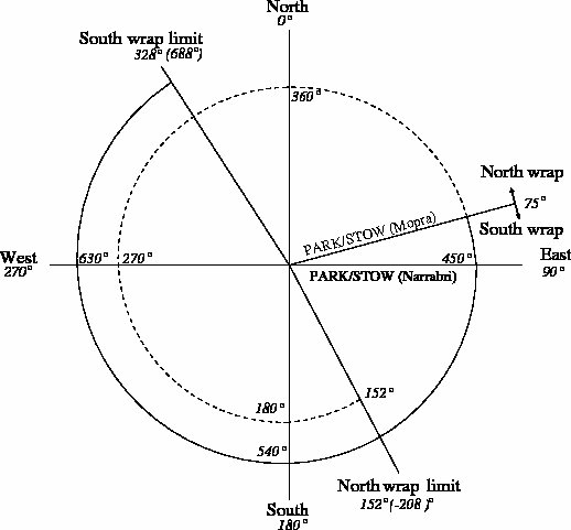
It is a good idea to check what wrap the telescope is in at the start of your observations, as “unwrapping” can take up to 10 minutes. To determine the wrap you are in, consult MoniCA or atdrivemon. MoniCA shows the wrap explicitly, on the “ATCA Summary” page. atdrivemon shows the azimuth using the ATCA convention — while in the South wrap azimuths are expressed as positive angles, and negative angles in the North wrap.
The CABB web scheduler is used to prepare schedule files. The web scheduler checks the schedule for completeness and, where possible, checks choices such as observing frequency for hardware compatibility. Drive times, and source azimuths and elevations can also be computed to enable you to estimate overheads and observability.
Three steps are involved in using the web scheduler:
A new scan is added to the schedule.
The details of the scan are changed as desired.
When all the scans have been defined, the entire schedule is written to file.
When constructing a schedule, consider:
Is the sequence of sources sensible, and how much time is expended on slewing?
Does the schedule contain all the sources, and at the appropriate frequencies and bandwidths?
The web scheduler can produce a listing to help answer these questions.
It is a good idea to study these listings very
carefully before observing commences. The scheduler considers drive times:
all coordinate entries are automatically followed by a calculation of the
azimuth and elevation of the source, as well as the drive time from
the previous source, using the entered value for LST. When making
a schedule file, the integration times are specified
for each source (and calibrator source). Note that,
except in the case of mosaic schedules and Dwell scan types,
these integration times
include drive times, so the specified time must be somewhat longer
than the amount of integration on source required. This is
particularly important for gain calibrators, when the drive time
(up to a minute or so) may be comparable to the integration time
(one to three minutes). Alternatively, the ScanType field can
be set to Dwell to ensure a source or calibrator
is tracked for the specified scan duration.
The schedule file submitted to caobs (the online Compact Array control
task) need have no specific start time. Rather, the schedule file asks
caobs to start the first scan as soon as possible. The sequence of
scans will be exactly as specified in the schedule file. However, when
using the web scheduler, the calculation of azimuths, elevations and drive times
is possible only if the starting sidereal time is known (at least
approximately). The sidereal time for the first scan in the schedule
can be set in the web scheduler by giving the time in the Time field,
and setting TimeCode to LST. Alternatively, the starting UT
may be specified by setting TimeCode to UT, and by setting
the Date to the appropriate start date by clicking on it and using
the calendar that appears. Note that when viewing any scan other than the
first in the schedule, the fields Time, TimeCode and
Date all become read-only.
The environment flag can be used to instruct the online software to remember certain settings, such as attenuators, and to recall them whenever a scan with the same environment flag is encountered. However, this is generally not required, as the online software will remember user settings, and recall them when the same conditions are encountered again. There are at least 128 slots for user settings, so for a normal schedule, the environment flag will probably not need to be used.
See Appendix F for a complete guide to all the functionality available in the web scheduler.
Yes! In this section a simple continuum schedule file is constructed. It will contain three sources: a program source and two calibration sources. The following observing sequence will be specified:
Setup calibrator (0537-441, a catalogued source) for 5 minutes,
Program source (R.A. 05:21:35.5, Dec. -21:24:27.1 (J2000)) for 30 mins,
A gain calibrator for 5 minutes.
These sources will be observed at the standard 4cm band frequencies of 5500/9000 MHz. To create this schedule file, perform the following steps (instructions are given in bold, and the results of the instruction, or important caveats, and described below it):
- Navigate to the CABB web scheduler in a web browser.
The first screen is displayed.
-
Change the
Sourcefield totest, theRAfield to05:21:35.5and theDecfield to-21:24:27.1. The delimiter for coordinates must be a colon, and the default
EpochofJ2000should only be changed if necessary.-
Change
ScanLengthto 00:30:00 and change theScanTypetoDwell. This ensures that 30 minutes are spent on source, regardless of slewing times.
-
Ensure
Pointingis set toGlobal. Offset pointing is not required for low-frequency observations.
-
Change the
Observerfield toWild, theProjectcode toC123. These fields should be set in the first source - they will propagate to the other sources as they are added.
-
Change the
Timefield to02:00:00, and theTimeCodefield toLST. This indicates that the schedule will be started at an approximate LST of 2h.
-
Click the
Freq1 Setupbar. This brings up the frequency selection fields.
-
Enter
5500in theContinuumfrequency box, and keep theChn. BWselection box to1MHz. The velocity resolution should be calculated to be 55 km/s, and the velocity range will be 111632 km/s.
-
Click the
Freq2 Setupbar. This brings up the frequency selection fields.
-
Enter
9000in theContinuumfrequency box, and keep theChn. BWselection box to1MHz. The velocity resolution should be calculated to be 33 km/s, and the velocity range will be 68219 km/s.
-
Click the
Scan Parametersbar. This brings up the scan details.
-
Click the
Search Calbutton. This presents a list of nearby calibrators to the right of the scan details, sorted by distance to the source. The closest source to the program source with a moderate flux density (> 1 Jy) is shown to be 0454-234, at a distance of 6.02°.
-
Click on the
0454-234button. The details for this source are displayed from the calibrator database below the source list. This source is a suitable gain calibrator as it has a decent flux density, has a defect less than 0.1% and a closure phase less than 0.3%.
-
Click on the
0454-234button again. Clicking on the button twice (without clicking another source button between clicks) inserts this source into the schedule above the currently selected source.
-
Select source 1, and change the
ScanLengthfield to 00:05:00. -
To copy this source to the end of the schedule, click on the
Editmenu and selectCopy, then select thetestsource, click onEditand selectPaste. The schedule should now have three sources (in order): 0454-234, test, 0454-234. The first source needs to be changed to 0537-441.
-
Select source 1
,
Change the
Sourcefield to 0537-441 and pressTAB. The scheduler will automatically put the source coordinates for this known calibrator in the
RAandDecfields.-
Click on the
Filemenu and selectSave As. The
Schedule file selectorwindow will appear.-
The schedule will be called c123_test.sch, so enter this into the
Filterbox to ensure that there is not already a schedule with this name. If there is another schedule with the desired name, consider changing it.
-
Enter
c123_test.schinto theSchedulebox and press theSavebutton. The file selection window will disappear, and the name of the schedule should now appear at the top of the window.
To produce a listing of the schedule, in order to check that the
schedule proceeds as expected, click on the Listing tab.
Yes! This example adds to the example from the previous section; ensure that the schedule created in the previous section is in the scheduler before continuing.
Now the aim is to observe 1 zoom band in each IF, each covering at least 70 km/s. The galaxy “test” is actually at an LSR recessional velocity of 25000 km/s, and these observations will look for CH3OH methanol and HC3N cyanoacetylene lines.
To create a schedule that can perform suitable observations for this situation, follow the steps:
- Select the first scan in the schedule.
This should be 0537-441.
-
Select the
Global changemenu item from theToolsmenu before changing theDateof this scan to 30/11/2014. The date that the observation will be performed is required to ensure that the observatory velocity is computed correctly.
-
Hit the
Global Applybutton. The date will now change for all the sources in the schedule.
-
Select the
Advanced viewmenu item from theToolsmenu. You should now see many more input fields.
-
Select the “
test” source in the schedule, then enter “25000” into theCatVelfield, and press TAB. The entry in the
CatVelfield should now read “25000 lsr radio” as the default frame is LSR, in the radio convention.-
Click the
Freq1 5500MHzbar. This brings up the IF1 frequency selection fields.
-
Click the topmost
Velobutton. This brings up the velocity calculator.
-
Select the
CH3OHline from theSpectral Linedropdown box. The rest frequency of this line (6668.518) appears in the
Rest Frequencybox below. TheSky Frequencywill be updated to 6112.092 MHz, and the zoom band frequency will be calculated as the nearest half-MHz, in this case as6112MHz.-
Click the
Applybutton in the velocity calculator. The velocity calculator will disappear and information will be inserted into the first zoom band. In this case, the
6112MHz frequency translates into the channel3273. The velocity resolution is given as 0.024 km/s, and the velocity range is listed as 49 km/s.-
Select the zoom band width to be
2from the width drop box. The velocity range now increases to 73.6 km/s.
-
Click the
Freq2 9000MHzbar. This brings up the IF2 frequency selection fields.
-
Click the topmost
Velobutton. This brings up the velocity calculator as before.
-
Select the
HC3Nline from theSpectral Linedropdown box. The rest frequency of this line (9098.332) appears in the
Rest Frequencybox below, and theSky Frequencywill be updated to 8339.161 MHz. The zoom band frequency will be calculated to be8339MHz.-
Click the
Applybutton in the velocity calculator. The velocity calculator will disappear and information will be inserted into the first zoom band. In this case, the
8339MHz frequency translates into the channel727. The velocity resolution is given as 0.018 km/s, and the velocity range is listed as 36 km/s.-
Select the zoom band width to be
3from the width drop box. The velocity range now increases to 71.9 km/s, comparable to the width provided for the IF1 zoom band.
-
Click the
Scan Parametersbar. This brings up the scan details.
-
Select the
Master1option from theFreqConfigdropdown box. This signifies that the frequency configuration, including the zoom modes, from this scan, should be defined as the master configuration.
-
Select the
0537-441source from the schedule, then elect theSlave-1option from theFreqConfigdropdown box. Now this scan will exactly mirror the frequency and zoom mode configuration from the
testscan, even if the configuration of thetestscan is changed. When a scan is set as a slave scan, theFreqpanels will display a message describing which frequency and scan it is slaved to.-
Select the
0454-234source from the schedule, then select theSlave-1option from theFreqConfigdropdown box. Now this scan will exactly mirror the frequency and zoom mode configuration from the
testscan.
At this point, the schedule would correctly describe a zoom mode observation.
The data rate during CABB observations can be calculated with the formula:
where
is the number of bytes produced per integration cycle,
is the number of bytes per correlation product, and
is the number of IFs,
is the number of channels in IF ,
is the number of Stokes quantities in IF ,
is the number of correlation products in IF ,
is the number of bins in IF , Stokes parameter and correlation product .
The data-rate per second is thus:
where the cycle time of the correlator.
A few example calculations are given below. In all cases it is assumed that bytes (in all modes, 4 bytes are recorded for each of the complex visibilities, and 4 bytes are recorded for the weight component), and seconds.
For a typical continuum observation, we have:
2 IFs (), each with
2049 channels (),
4 Stokes parameters (XX, YY, XY, YX; ),
21 correlator products (6 auto-correlation and 15 cross-correlation spectra; ).
Each auto-correlation same-polarisation (XX, YY) spectrum has 2 bins (noise diode on and noise diode off; ).
Each auto-correlation cross-polarisation (XY, YX) spectrum has 1 bin ).
Each cross-correlation spectrum has 1 bin ().
Putting this in Equation 2.3 we get
This works out to be a data rate of 0.300 MiB per second, or roughly 1.055 GiB per hour. Note: we use the binary prefixes MiB and GiB (the mebibyte and gibibyte) for data sizes. See Wikipedia for a good explanation.
Since CABB data files will automatically close when they reach 4.0 GiB in size, it would take approximately 3 h 47 m to fill one file (not accounting for the overhead consumed by the header information).
For an observation where each of the 16 zooms in each IF is recorded, and no zooms are consolidated, we have:
34 IFs (). Two of these are the continuum IFs, each having
2049 channels (),
4 Stokes parameters (XX, YY, XY, YX; ),
21 correlator products (6 auto-correlation and 15 cross-correlation spectra; ).
Each auto-correlation same-polarisation (XX, YY) spectrum has 2 bins (noise diode on and noise diode off; ).
Each auto-correlation cross-polarisation (XY, YX) spectrum has 1 bin ).
Each cross-correlation spectrum has 1 bin ().
The other 32 IFs are the zoom bands, each having
2049 channels (),
4 Stokes parameters (XX, YY, XY, YX; ),
21 correlator products (6 auto-correlation and 15 cross-correlation spectra; ).
Each spectrum has 1 bin ().
Putting this in Equation 2.3 we get
This works out to be a data rate of 4.352 MiB per second, or roughly 15.3 GiB per hour. Since CABB data files will automatically close when they reach 4.0 GiB in size, it would take approximately 15 m to fill one file (not accounting for the overhead consumed by the header information).
For an observation using CABB's pulsar-binning mode, we have:
4 IFs (). Two of these are the normal continuum IFs, each having
2049 channels (),
4 Stokes parameters (XX, YY, XY, YX; ),
21 correlator products (6 auto-correlation and 15 cross-correlation spectra; ).
Each auto-correlation same-polarisation (XX, YY) spectrum has 2 bins (noise diode on and noise diode off; ).
Each auto-correlation cross-polarisation (XY, YX) spectrum has 1 bin ).
Each cross-correlation spectrum has 1 bin ().
The other two IFs are the pulsar-binned continuum bands, each having
513 channels (each of them being the average of 4 of the normal continuum channels) (),
4 Stokes parameters (XX, YY, XY, YX; ),
15 correlator products (15 cross-correlation spectra; ).
Each cross-correlation spectrum has 32 bins across the pulse period ().
Putting this in Equation 2.3 we get
This works out to be a data rate of 1.803 MiB per second, or roughly 6.339 GiB per hour. Since CABB data files will automatically close when they reach 4.0 GiB in size, it would take approximately 37 m to fill one file (not accounting for the overhead consumed by the header information).
Since all modes give you the continuum IFs, you start off with one of two base data rates, per cycle. For the 1 MHz modes, the base data rate is:
bytes per IF. For the 64 MHz modes, the base data rate is:
bytes per IF.
For each pulsar-binned IF you have (only available in 1 MHz mode) you add:
For each single zoom you have (i.e. zooms with a width of 1) you add:
For each consolidated zoom you have (i.e. zooms with a width of 2 or more) you begin by adding:
Then, for each zoom band in the consolidated zoom, you add:
For example, if you had a consolidated zoom with a width of 5, it would produce
bytes per cycle.
Example: If you were using the 1 MHz/64 MHz hybrid CABB configuration, and had one zoom of width 1 and one consolidated zoom of width 12 in the 64 MHz IF your total data usage would be:
Doing the sum gives bytes per cycle. Assuming a 10 second cycle time, this would generate 3.997 GiB per hour, which would give you roughly one new CABB data file every hour.
Users of the ATCA are expected to organise the execution of the observations. Any member of the team that proposed the experiment is eligible to observe from the Marsfield SOC, or any other researcher that the primary investigator might like to nominate. If the researcher has not previously observed with the ATCA and CABB, or has not observed within the past 12 months, they will have to travel to the SOC to be trained.
Yes. It is recommended that observers unfamiliar with the ATCA arrive at the SOC at least two full weekdays before their observations, in order for them to become familiar with how to use the array and who to talk to if things go wrong.
If it is not possible for any of your team members to come to the SOC for your allocated observing time, but you have visited SOC sometime in the 12 months prior to your observations, you may be granted permission to do your observations remotely (Section 2.4.4).
We expect that observers are members of the team that proposed the experiment. Said another way, if you require someone to do your observations, we fully expect that that person would become a collaborator, and would be included on any publications derived from those observations. If this is what you require, you will need to alert ATNF staff well ahead of your scheduled time (4 weeks at least).
We understand that plans can change on short timescales and without warning. We recommend first trying to recruit another member of your team to do the observations, but should that not be possible, please alert ATNF staff.
It may be possible to do a short-notice scheduling swap with another project, leaving you to do your observations at a later date. If this is not possible, we may be able to find a replacement observer, with the understanding that whomever does the observing will become a collaborator on the experiment, and will receive due credit on any publications derived from the observations.
Remote observing is available for experienced ATCA observers. We will consider granting a request for remote observations if the observer:
Has observed from the SOC at least once in the 12 months prior to the date of the proposed remote observations, or
Usually observes more than 3 times per semester, or on at least 10 days per semester, and has observed from the SOC at least once in the 18 months prior to the date of the proposed remote observations.
Applications to do a remote observation must be made at least 2 weeks before the observations. This is so observatory staff can check for possible network disruptions during your observations, and advise you if remote observing will not be possible. The later you leave your remote observing application, the less time you will have to change your plans should your request for remote observations be refused.
Permission to do your observations remotely is given at the discretion of science operations staff, and you should not presume that permission will be forthcoming. Should permission be refused and you are not able to come to the observatory, you may need to find a local collaborator to do the observations for you. The duty astronomer is under no obligation to observe for your project if you are unable to.
To apply to make an observation remotely, use the “Booking” tab on the ATCA observing PORTAL, which will look something like Figure 2.2. To book for a slot, click on the start time and then drag out a box to the end time of the booking. A booking box will pop up, and you can adjust the start and stop times if you need to.
Remote observers must have their own ATNF UNIX account and remember their password for this account.
To be sure of a successful remote observing session, all observers are required to test their remote observing setup at least a week before their observations.
At a minimum, you will require the following for remote observing:
A computer with SSH software, capable of running a VNC viewer, on a high bandwidth connection,
A telephone near to the computer, that can make calls to, and accept calls from the observatory.
Remote observations will be easier if you also have:
Two or more monitors attached to their computer,
A computer with X-Windows software,
A hands-free speakerphone or headset.
To test your setup, you should contact the duty astronomer and ask to be allowed to login and perform the test. If the test will not disturb current observations, you should follow the instructions on remote observing found in Chapter 3 to ensure that you can monitor and control all the required VNC sessions. If problems are encountered here, and the duty astronomer can't help you resolve them, contact the observatory staff with a description of the problems and ask for advice.
In the 2017APR semester, a rapid response mode was introduced. This is designed to allow the ATCA to respond almost instantly to a request for a NAPA over-ride. This section describes how to use this mode.
The ATCA rapid response mode is only available to proposers who have submitted a
NAPA proposal for the current semester. If you are interested in being granted
permission to use the rapid response mode for your NAPA proposal, please talk
to Jamie Stevens (<Jamie.Stevens@csiro.au>).
The rapid response mode is designed to take a user-made schedule, and get it onto the telescope as soon as possible after the request has been made. Getting the telescope to stop one schedule and start another is very easy; determining when "as soon as possible" actually starts is the tricky part. The rest of this section describes the process which takes place to perform an over-ride observation.
You submit a NAPA science case to the ATNF TAC, which gives you a ranking grade for the semester.
You ask for, and are supplied with an authorisation token which will allow you to request an over-ride through the rapid response service.
At some point during the semester, you decide to trigger your NAPA proposal. You (or more likely your software) creates a CABB schedule that observes both the target of interest and a nearby gain calibrator.
You submit this schedule to the ATCA rapid response web service.
The service checks that you are an authorised user, and rejects the request if not.
It then checks that the minimum amount of time that you have requested is still available to be scheduled for your project, considering the amount of time you requested from the TAC, and the amount of time you have used before this request. If you do not have sufficient time, the request is rejected.
A start time is determined where the source is above the ATCA lower elevation limit, and that the schedule can be executed for at least the minimum required amount of time while still being above the horizon. The search for this suitable start time is limited to either 100 hours after the request submission, or to a user-specified duration, if it is less than 100 hours. The 100 hour limit is designed to allow for an automated response even for long weekends where the proposers may not be available for a manual over-ride, while the user-specified duration can indicate that an observation that can't be made within some time frame would no longer be scientifically interesting.
If a suitable start time cannot be found, the request is rejected.
An estimate is made of when the flux-density and bandpass calibrators should be observed, given the start time. The schedule is altered to insert those scans.
If the request has not been rejected by this point, the request is approved.
At the start time determined in the previous step, several additional checks are made.
All scheduled scans will be above the ATCA lower elevation limit at their expected start time, for at least the minimum required time.
The array is not stowed due to weather conditions.
CABB is configured in either 1 MHz continuum mode, 1 MHz zooms mode, or 64 MHz zooms mode.
If any of these conditions is not met, then the start time of the project is delayed from between 5 seconds and 10 minutes, at which point each of the checks are made again.
When all checks from the previous step are satisfied, a final set of schedule alterations are made.
The schedule is shortened if necessary, to fit in the time available at this start time. The amount of time scheduled will always be at least the minimum required.
If the user has requested to use the same frequency configuration as the project being over-ridden, and
the band currently being observed (or that was last observed) is not 7mm or 3mm,
the array is not currently split between two bands,
and the project that is currently being observed (or that was last observed) is not C999,
then the over-ride schedule is altered to use the same frequency configuration as is currently listed. Otherwise, the frequency configuration is left as specified in the request.
If the slew from the current position to the first scan of the schedule is less than 20 seconds, and the delays need to be reset because the user-specified frequencies are being used instead of the currently configured frequencies, an additional “Normal” scan of 40 seconds is inserted at the beginning of the schedule. This scan is named “setup” so it can easily be identified and discarded during later data reduction.
The first scan in the schedule is altered, in the following ways.
The command
focus defaultis added, to ensure the focus is set correctly.If the scheduled frequencies are not the same as those that were observed before the over-ride, the command
corr reset delaysis added, and the tv-channels are set to be 1020 to 1022 in each IF.
If CABB is currently configured in 64 MHz zooms mode, several scans are added at the beginning of the schedule to do an automatic delay calibration for the user-specified frequencies. A description of how this is done can be found at this link.
The altered schedule is copied into the right place, caobs detects this new schedule file and immediately begins executing it. Over-ride schedules are started at scan 1, and continue through until the last scan, and will not loop.
While the schedule is being executed, an automatic monitoring system will watch that the schedule is progressing, and will attempt to automatically restart the schedule in the event that it gets stopped.
All scheduled slots that have a project code starting with “C” can be over-ridden by the rapid response mode, provided that your TAC score is sufficiently high and CABB is in the correct mode.
Blocks of time scheduled for reconfigures, maintenance and VLBI cannot be over-ridden.
Any over-ride project that has a score higher than or equal to the lowest score given to a scheduled project may over-ride any other scheduled project. The theory for this is that if we knew at the beginning of the semester when a NAPA would trigger, and that NAPA had a score about the lowest score that was actually scheduled, we would have attempted to schedule it at the appropriate time and scheduled the displaced project at another time, regardless of the score of the displaced project.
As part of the project to develop this rapid response mode, a library for creating and manipulating CABB schedules was developed. It can be found on GitHub, and is free for use.
Because many of the existing libraries that astronomers use to deal with transient event streams are written in Python, the choice was made to focus first on providing a Python library for schedule manipulation. This library is targetted toward Python 2.7, but will work with 3.8.
Documentation on how to use the library in your own code is part of the GitHub repository.
To ensure that only those projects that have been pre-approved can perform over-rides on
the ATCA, any request for over-ride time needs to be accompanied by
a valid authorisation token. This can only be obtained by emailing
<Jamie.Stevens@csiro.au>.
There are two types of authorisation token available. The first is a test token, which allows you to submit a request, and go through the entire process of the over-ride, but not actually get time on the telescope. This is designed to be used while you are trying to develop and perfect your automated trigger routines. You may issue as many requests as you like with a test token.
The second token will allow your request to allocate time on the telescope. This type of token will not be issued until you have demonstrated that your code can properly submit a test request. You will need to work with Jamie Stevens during this process.
Authorisation tokens are valid only for a specific project and semester, and will be rejected if used outside those bounds.
The authorisation token itself is a JSON Web Token. You will be supplied with a normal ASCII file that will need to be passed back to the service whenever you make a request.
All requests to trigger an over-ride observation are submitted through a web service. The exact format of the request won't be documented here, and we suggest that you use the Python code we provide when you are building your trigger response software.
The library which makes it easy to submit over-ride requests can be found on GitHub, along with documentation and examples.
If your request is unable to be scheduled given the bounds you provided, you will receive your rejection in the response from the web service.
If the web service doesn't reject your request, your schedule will enter the queue to be executed. At this point, two emails will be sent to this effect. As with all emails sent by the rapid response service, they will be from Jamie.Stevens@csiro.au and will go to all the members of the NAPA team (as specified on its OPAL coversheet), along with all the members of each project that will need to be displaced.
The first email will have the subject “ATCA rapid response mode triggered for Cxxxx ”, where of course the real NAPA project code will be specified instead of “ Cxxxx”. The second email will have the subject “Your ATCA rapid response over-ride request has been queued for execution.”.
The first email will look something like this.
The ATCA rapid response mode was requested by the NAPA project C008 at UTC 2017-03-31 04:14:14.
This over-ride has been scheduled to begin at UTC 2017-03-31 04:14:14 and end at approximately UTC 2017-03-31 04:27:06.
This over-ride has been assigned the ID xaap6yuacy10ltg9lc3g.
This will displace time from the project C007.
The observations will be automatically started without any user intervention. While the observations are running, please do not intervene unless advised to by observatory staff.
You will receive another email when the observations have started, and another when the over-ride observations have ended. Messages to the same effect will also appear in the ATCA Portal chat.
Please send any feedback about this system by replying to this email.
As you can see, the time of the request, and the expected start and end times are all listed, along with the unique ID assigned to the over-ride, and a list of all the projects that will be displaced.
The next email will look similar to the following.
This email is from the ATCA rapid response system.
What follows is a log of the progress of your requested over-ride experiment.
Project code: C008
Over-ride ID: xaap6yuacy10ltg9lc3g
2017-03-31_04:14:14: Your experiment has been placed in the queue, and should start at 2017/3/31 04:14:14. You will receive another email at that time.
If you have any concerns about this experiment, please reply to this email.
This second email introduces the time-stamped log of the progress of the over-ride. All subsequent email communication will contain this log, as it was when the email was sent. The log will have entries for all the important actions made by the rapid response service, and entries that will be useful for later data reduction.
At the start time, the service will either start or delay the schedule, and in either case an email will be sent. If the schedule is started, the email will have the subject “An ATCA rapid response over-ride is now being observed”, while if the schedule is delayed the subject will be “Your ATCA rapid response over-ride request has been delayed”; the reasons for the delay will be included in the log. If the schedule is started, the name of the schedule will be given in the email, and you may load it in the CABB web scheduler to see how the service has altered it.
No emails will be sent while the schedule is running, except if the service encounters a problem. In that case, you will get an email with the subject “There has been a problem while executing your ATCA rapid response over-ride”.
When the schedule finishes, the service will send out one final email, with the subject “ATCA rapid response over-ride is now complete”. This email contains the full log, which will include the name of the RPFITS files that contain the data.
If for some reason the service is unable to perform the scheduled over-ride (for example, if the antennas are weather stowed for an extended period of time), then the schedule might expire and be removed from the queue. If this happens you will get an email with the subject “Your ATCA rapid response over-ride request has expired”.
The schedule you make depends on what type of observation you are trying to perform. What follows are some general recommendations for rapid response schedules.
Select the frequencies that will give you the best science, rather than ask for the frequency configuration that is being used when the telescope is over-ridden. There is no actual need to have a perfectly calibrated array when doing an observation with the ATCA. As long as the delays can be measured while observing a strong calibrator, you will be able to correct for those delays in Miriad. If you specify the frequencies you want, the service will ensure that the delays are set back to their defaults at the start of your observation, which will always produce a dataset that can be successfully calibrated.
To ensure that the observations can be monitored effectively with default delays, the tvchannel range is limited to 1020 - 1022 in each IF. This 3 MHz of bandwidth near the band centre is sufficient to measure the system temperature and to show the calibrator's flux density in vis. You will not need to specify this when creating the schedule, as the service will automatically do this for you.
If measuring very early prompt emission is important to your science, ensure that you visit the target source first, before your first scan on the gain calibrator. Observing your target for a few minutes before going to the gain calibrator should not be a problem, as the gains can be reliably extrapolated at cm wavelengths. Also, if you are observing in the 16cm band, there is a very good chance you will have a source in your field that is bright enough to allow for self-calibration.
Keep your scans short so the service can easily cut it to fit the earliest available slot. If authorised to do so, the service can automatically shorten the schedule you provide in order to fit it into the earliest possible available slot; how it does this is described in Section 2.5.9. If you keep your scans short (ie. don't have hour long scans between visits to your calibrator) then the shortener will act much more reliably.
Do not include a flux density calibrator in your schedule. The service will automatically add the appropriate flux density calibrator to your schedule, depending on frequency and sidereal time.
The service shortens a schedule in four stages.
The hard end time of the available slot is determined. This may be because the source has set, or some sort of maintenance or reconfigure is scheduled. All scans that end after that hard end time are immediately deleted from the schedule, except if it is the flux density calibrator scan that the service added.
As mentioned in Section 2.5.8, this step can cause problems if your scans are too long. Consider a scenario where the scan that ends after the hard end time is scheduled to run for 1 hour. Even if the hard end time is only 10 minutes from the scheduled end of this scan, the entire scan is cut, and you have lost a potential 50 minutes of observing time.
If the schedule is still too long at this point, all scans on the nominated calibration source may be shortened to have a dwell length of 1 minute. This is done from the first scan and continues until all the calibrator scans have been shortened, or the schedule now finishes before the hard end time.
If the schedule is still too long at this point, then the scan on the flux density calibrator is shortened by 1 minute.
If the schedule is still too long at this point, then the source scans are shortened. The service calculates the amount of time that needs to be cut for the schedule to fit in the slot, and then subtracts as much time as possible from the last remaining source scan. If the last remaining source scan is longer than the cut time, then the scan survives, otherwise it, and the following calibrator scan, are removed entirely. This process repeats until the schedule finishes before the hard end time.
If at the end of this process, the schedule length falls below the specified minimum useful time required, the start time will be delayed and the schedule restored to its original specification.
Ready to observe? Check that all the following tasks have been done:
Determined sources to use for:
Delay calibrator
Flux density calibrator
Bandpass calibrator
Gain calibrator(s)
Pointing calibrator(s) (only if doing reference pointing)
Polarisation calibrator(s) (only if doing polarisation studies)
Checked that all sources are visible during allocated time.
Prepared a schedule file using the CABB web scheduler for:
Array setup
Calibration
Science observations
Used the sensitivity calculator to make sure that integration time on calibrators is sufficient.
Ensured that turret movements are limited to once every 15 minutes or longer.
Generated a mosaic pointing file (only if doing mosaic observations), and copied it to the appropriate place on xbones.
Generated an ephemeris for the solar system object (only if doing solar system observations), and copied it to the appropriate place on xbones.
Calculated how much data the observations will generate, and obtained enough disk space to accommodate this.
Checked for possible problems, and made contingency plans for:
Antenna shadowing
Wrong time range for flux density calibrator observations
Bad weather forecast during observations
Checked the Portal for issues that may cause problems with the observations.
Checked that remote observations are permitted (only if remotely observing).
Contacted observatory staff and duty astronomer if assistance will be required during observations.
| Revision History | ||
|---|---|---|
| Revision 1.8 | 2022 April 20 | jbs |
| Add CABB block reboot figure back into the troubleshooting section. | ||
| Revision 1.7 | 2021 October 19 | jbs |
| Remove link to remote observing web page, and update other links. Changed advice on sampler levels. Fixed description of how CABB calculates delays. Fixed description for heat stow trigger conditions. Split the very long flowchart for the printed output. Remove info on how to configure Twitter for SMS, since that is no longer available. | ||
| Revision 1.6 | 2018 June 21 | jfk, ghh |
| Substantial updates to content | ||
| Revision 1.5 | 2018 March 15 | jbs |
| Add a section describing unattended observing, and update information on PMon wind stows | ||
| Revision 1.4 | 2016 May 31 | jbs |
| Document how to use the ATCA alarm Twitter feed | ||
| Revision 1.3 | 2015 Nov 24 | jbs |
| Add description of how to set CABB attenuators for 16cm | ||
| Revision 1.2 | 2015 Oct 23 | rmw, sb, klw |
| Substantial revision of content and layout | ||
| Revision 1.1 | 2014 Jul 09 | rmw |
| Substantial revision of content and layout | ||
| Revision 1.0 | 2014 Mar 20 | jbs |
| Initial Docbook revision | ||
This chapter describes the steps necessary to observe with the ATCA. It assumes that observing strategy has been determined and schedule files created. See Chapter 2 for information on determining observing strategy and Section 2.3 for information on creating schedule files.
In general, observing takes place in the SOC in Marsfield. It is possible to remote observe from anywhere with adequate network and phone connectivity.
We are currently in the process of creating ATCA Tutorial videos that are available on our YouTube channel. These videos are intended to help new observers familiarise themselves with the various applications and operational processes related to the ATCA and are provided as “refresher courses” for more experienced observers.
Observers are responsible for the collection of their own data and appropriate checks to ensure the quality of the data. They are also expected to ensure the safety of the array (to the best of their ability). This is always secondary to any personal safety concerns.
An ATNF staff astronomer or student is rostered to support observers with setting up and training new observers to use the array (the Duty Astronomer or DA). The DA should be the first point of call if there are problems or queries with observations.
The steps to observe with the compact array are:
connect to VNC sessions and prepare for observing (Section 3.1)
taking control from the previous observer (Section 3.2)
set up and calibrate the array (Section 3.3)
observe target source(s) (Section 3.4)
monitor observations for problems (Section 3.5)
end observations
When observing remotely, getting connected can take a while so observers should make sure that they leave plenty of time before their observing block begins.
Before the start of observations, observers need to log into the ATCA Portal.
Two VNC sessions are set up for control of the array:
The xbones session runs caobs, vis and assistance.
The caccc1 session runs tasks associated with the correlator.
Remote observers should connect to both of these VNC sessions before the start of observations. See for information on setting up remote observations (In Marsfield the necessary windows are already set up on Ara in the SOC, along with a number of additional windows with supplementary information and observing tasks.)
When it is time to take over, check on the portal and chat with the previous observer or observatory staff and ask if it is ok to get going. The Duty Astronomer should be on hand to help inexperienced observers set up their observations.
The main observing program that the observer interacts with is caobs.
caobs usually runs in a black screen with yellow writing in the xbones
VNC session. The program cacor is the interface to the correlator. cacor
commands can be executed for caobs by prefixing the command with corr [command].
Other programs that observers need to use include spd, vis and MoniCA.
For details on using these programs see Appendix A, Appendix B, Appendix C, Appendix D and Appendix E.
To start observing, load a schedule with a strong calibrator into caobs and drive to the source:
caobs> set file
| loads the schedule file | |
caobs> track # | drives the telescope to scan # in the schedule file |
At the start of observing, a number of procedures need to be executed to set up the array for observng. The following table summarises the tasks, and indicates the wavelengths which need the various tasks.
| 16cm | 6&3cm | 15&7mm | 3mm | ||
| Set focus | ✔ | ✔ | ✔ | ✔ | See Section 3.3.1 |
| Set CABB attenuator levels | ✗ | ✔ | ✔ | ✔ | See Section 3.3.2 |
| Set CABB channel ranges | ✔ | ✔ | ✔ | ✔ | See Section 3.3.3 |
Check delavg | ✔ | ✔ | ✔ | ✔ | See Section 3.3.4 |
| Flag interference | usually not necessary | See Section 3.3.5 | |||
| Calibrate delays | ✔ | ✔ | ✔ | ✔ | See Section 3.3.6.1 |
| Check pointing | ✗ | ✗ | ✔ | ✔ | See Section 3.3.6.2 |
| Calibrate phases | ✔ | ✔ | ✔ | ✔ | See Section 3.3.6.3 |
| Calibrate gains | ✔ | ✔ | ✔ | paddle | See Section 3.3.6.4 |
The subreflector on each of the ATCA antennas can be raised and lowered to allow the signal to be focussed at the receiver feed. However, changing the subreflector position will change the path length (obviously) which will change the geometric phases and delays, so, it should only be done when required, usually when the frequency changes. Extra care is needed with calibration with programs that change focus during the observation.
A good time to do this is at the start of the observing and it can be done while driving to source.
Default focus positions have been determined for each band.
caobs> focus default | drives the subreflector to the default focus height for that band | |
caobs> focus ca0# | drives the subreflector on antenna # to the given focus height in mm |
Table 3.1. Subreflector Focus Positions for the Antennas.
| Ant | 16cm | 4cm | 15mm | 7mm | 3mm |
|---|---|---|---|---|---|
| CA01 | 17.0 | 4.1 | 17.8 | 17.0 | 14.0 |
| CA02 | 10.0 | -1.9 | 10.7 | 9.8 | 10.0 |
| CA03 | 10.0 | -2.2 | 10.4 | 9.0 | 9.0 |
| CA04 | 23.0 | 10.6 | 23.0 | 23.0 | 23.0 |
| CA05 | 18.0 | 7.1 | 20.2 | 18.5 | 18.4 |
| CA06 | 22.5 | 7.0 | 20.5 | 22.5 | 22.5 |
Note: As the antenna tips over, it deforms slightly, and the detected focus position changes by up to 1mm. This is normal and will not significantly affect the data.
The rms digitiser quantisation levels (as displayed in the
sampler tab of cacor; see Figure 3.2) should be close to 20
(Range: Approximately 15-25).
To set the levels, attenuation can be added or removed.
The values in the Atten section of the window show the settings of the cacor
attenuators. They have a range of 0-15 dB.
For 16cm observations, strong RFI in the band will often make the sampler levels vary
significantly from cycle to cycle, making it difficult
(and often impossible) to set the attenuators appropriately.
It is therefore recommended to skip this step when observing at 16cm.
However, in rare cases the attenuator settings shown in the Atten section
could be quite low (all values far below 7), and at those times it could be useful to reset them either
automatically or manually as described below.
For all other bands, if the levels are not close to 20, the ATTS button in the cacor GUI can be activated to enable cacor to automatically add or remove attenuation.
This can also be done in the cacor interface:
cacor> tatts[ervo] 20 | set the target for the attenuator servos to 20 | |
| (most of the time, this command is not needed as tatts will usually already be set to this level) | ||
cacor> atts[ervo] on | correlator servos the attenuators to adjust the levels into the samplers |
Wait for the levels to settle to around 20, then turn the adjustment off again with:
cacor> atts[ervo] off |
Fairly obviously, the algorithm is unable to “improve” the levels if the attenuators are at their limits (0 or 15).
As noted above, strong RFI in the 16cm band makes it difficult to set the attenuators appropriately.
High values of attenuator settings, even up to the maximum value of 15, are not harmful.
However, you can also set the attenuators manually to values that
are known to be good, as listed in Table 3.2. To set the attenuators manually, you will need to
use the att command. For example, to set the CA03 attenuators as per Table 3.2,
you would need to give the commands:
cacor> att1 ca03 6 13 | sets the CA03 IF1 A and B pol attenuators | |
cacor> att2 ca03 2 2 | sets the CA03 IF2 A and B pol attenuators |
See
att
for more complete information about how to use this command.
f ca0# n m
Table 3.2. Attenuator settings for the 16cm band
| Product | CA01 | CA02 | CA03 | CA04 | CA05 | CA06 |
|---|---|---|---|---|---|---|
| 1 A | 5 | 4 | 6 | 7 | 8 | 6 |
| 1 B | 9 | 3 | 13 | 5 | 9 | 8 |
| 2 A | 10 | 4 | 2 | 9 | 8 | 4 |
| 2 B | 7 | 4 | 2 | 5 | 9 | 4 |
If the sampler levels are very low (approx 0), there is probably a problem which will need to be checked.
There are another set of attenuators in the receivers (as opposed to the correlator) which can also be used to set the levels.
These are controlled from caobs.
caobs> show atten[uation] | shows the current receiver attenuation levels in the caobs status window |
caobs> set atten ca0# atta attb | sets the receiver attenuator levels on antenna # to attenuator levels a and b. This value will be the same for both IFs. |
cacor generates an average visibility (either the mean or the median across the spectrum) that is used for Tsys and array calibration. In general, the median is much more stable and allows for a more reliable calibration. Otherwise, care needs to be taken to ensure that the range of cacor channels used for calculating the average is as wide as possible within the useable passband, but also excludes interference.
The default behaviour is to compute the average across the spectrum. To ensure that the more stable and reliable
median is being used, it is recommended to enable the tvmedian option:
cacor> tvmedian on on | Two arguments are required to enable the median option for both frequencies. |
At higher frequencies and when the tvmedian option is enabled,
it is usually appropriate to use the central fifty percent of channels.
The easiest way to do this is to type
cacor> tvch[an] default | sets the channel range to use the central 50% of the channels (i.e. channels 513 - 1537). |
Alternatively if tvmedian is disabled (not recommended), the information below can be
referred to.
At cm frequencies, interference means that it is often better to select
non-default channels, when tvmedian is disabled (not recommended).
See Table 3.3 for information on recommended channel ranges for 2048 MHz continuum bands.
If these channel ranges are not generating the anticipated visibility in vis, inspect Appendix C to
determine the cause of the problem.
The tvchan command sets the range of channels that are used for
calibrating the array and for Tsys calculation. The same range is used to
compute the average (or median) visibility for display in vis. All unflagged
channels are written to the data (RPFITS) file regardless of what the tvchan
setting is.
(Note: Channels that are flagged are written to the file as zeroes. See Section 3.3.5 for more information).
Current settings are displayed in the cacor GUI, as shown in Figure 3.3.
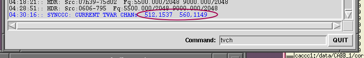
It is also possible to check the current setting with the cacor command
cacor> tvch[an] | The first pair of numbers gives the channel range for the first frequency. The second pair of numbers gives the channel range for the second frequency. |
Setting the range is done with the cacor command:
cacor> tvch[an] default | sets the channel range to use the central 50% of the channels (i.e. channels 513 - 1537). | |
cacor> tvch[an] ch1
ch2
ch3
ch4 | sets specific channels where ch1 and ch2 are the low and high channels for frequency 1 and ch3 and ch4 are the low and high channels for frequency 2. | |
cacor> tvch[an] f# ch1 ch2 | sets specific channels for a single frequency, where # is the frequency (1 or 2). |
Table 3.3 lists the suggested tvchan ranges for the standard continuum bands. On any given day (or interference environment) other ranges may be more appropriate.
Table 3.3. Suggested tvchan ranges for standard ATCA Continuum bands.
| Band | Centre Freq | 1 MHz channels | 64 MHz channels | ||
|---|---|---|---|---|---|
| (MHz) | ch1 | ch2 | ch1 | ch2 | |
| 16cm | 2100 | 200 | 949 | 2 | 14 |
| 6cm | 5500 | 513 | 1537 | 9 | 25 |
| 3cm | 9000 | 200 | 1149 | 9 | 25 |
| 15mm | 17000 | 513 | 1537 | 9 | 25 |
| 7mm | 33000 | 513 | 1537 | 9 | 25 |
| 3mm | 93000 | 513 | 1537 | 9 | 25 |
(There is a wide range of valid frequency settings at mm frequencies).
To calculate the delay of an individual IF, cacor
checks the phase in each channel in the tvchan range
(just defined) and calculates an average linear slope from
the phase measurements as a function of frequency; this slope is the delay.
If the noise on the phase is high (due to a faint source or poor weather, for example)
or there is some strong unavoidable RFI in the tvchan
range, then the average slope may not accurately represent the real
slope due to the delay.
To reduce the noise, or to average out the effect of the RFI, setting delavg in the correlator
averages together (or takes the median of) the corresponding number of channels in the
tvchan range before calculating the slope to determine the delay.
Here too it is useful to use the median option rather than the default mean (computed within each
group of delavg channels):
cacor> tvmedian on on | Two arguments are needed to enable the median option for both frequencies. |
Higher values of delavg can be useful for determining the delays.
However, care needs to be taken when selecting this value!
If the phases are wrapping quickly, averaging over a
large number of channels will give a meaningless average phase, and therefore incorrect
delays will be determined.
The current value of delavg is in the status bar of the cacor interface.
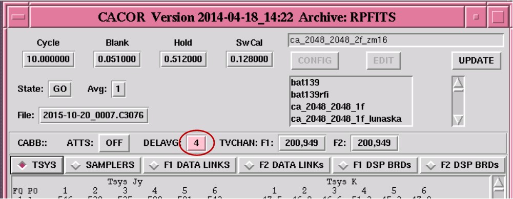
Setting delavg is done with the cacor command:
cacor> delavg # | Averages # channels. |
|
|
| |
|
An spd plot demonstrating slow changes in phase.
The phases are not wrapping at all in the A pol, and wrapping approximately every 250 channels in the B pol.
Averaging over 32 channels would still provide enough points across the band to achieve a useful linear fit to the data, so |
An spd plot demonstrating rapidly wrapping phases. The phases in both pols of this graph are wrapping across a small number of channels. It is possible to check just how quickly the phases are wrapping by viewing a smaller number of channels:
spd
The value of |
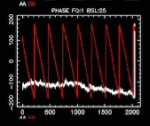
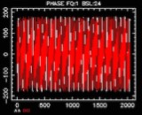
Occasionally, there will be channels that, because of interference (or other issues), you may wish to completely excise from the data (i.e. not write those channels to the data file).
To check the extent of currently flagged channels:
cacor> fflag | display the number of channels that are currently unflagged. In each frequency, there is a maximum of 2049 channels. |
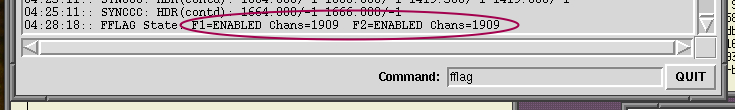
There is no easy way to discover which channels have been flagged, and flagging will remain even with a change of project (or frequency etc.) so flagging should be checked at the start of observing. If there are more channels flagged than anticipated, flagging should be cleared then reflagged if necessary.
This is done by:
cacor> fflag f# default | flags the central channel (and 1/4, 3/4 channels) in frequency # |
To flag the set of known bad continuum channels
cacor> fflag f# birdies | flags channel known bad channels in frequency # |
This needs to be done at both f1 and f2.
To flag explicit channels, use the command:
cacor> fflag f# chm | flags channel chm in frequency # | |
cacor> fflag f# chm-chn | flags channels chm to chn
inclusive in frequency # |
Again, this needs to be done at both frequencies.
If you know exactly which channels have been flagged, they can be unflagged with the
funflag command: formats are similar to the fflag command i.e.
cacor> funflag f# chm | unflags channel chm in frequency # |
Once the array is working, the system can be calibrated.
Calibration will not fix a broken system.
The calibration involves calculating and applying the delay offsets, checking the pointing (for mm observations), setting the phases to zero degrees and correcting the visibility amplitudes to the appropriate flux levels.
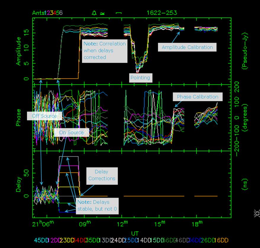
Delay offsets need to be determined and corrected at the start of the observation. Failure to correct for delay offsets may result in decorrelation, and loss of data.
In the 64MHz zoom configuration, delay calibration is more complex as it generally needs to be done in two steps. (First delay calibrate a zoom channel, then in the continuum. See Section 3.3.6.1.1 for more information)
To calibrate the delays, track an unresolved source with large flux density
(e.g. PKS1934-638 or PKS0823-500 for cm
observations; for mm observations use PKS1253-055,
PKS1921-293, PKS2223-052 or
PKS0537-441).
PKS1934-638 and PKS0823-500
do not have enough flux density to calibrate at mm frequencies.
Correlation should be apparent before you proceed. Phases in spd should be stable, though they may be wrapping rapidly and delays should be flat in vis. Check that you have correlation in both frequencies and both polarisations.
If there is significant interference (see the amplitude plot in spd), you will need to carefully craft the tvchan range (or, if bad enough, actually flag interfering channels) to avoid the interference in the calibration data.
If working at 3mm or with significant interference, it may be necessary to average over several channels (to improve the signal/noise ratio) with the command:
caobs > corr delavg # | where 8 is a good initial value for # - however,
if the delays are large (>50nsec), you should try a smaller value to start with. |
If you still don't have correlation, check Section 3.5.6 at the end of this chapter, and if this doesn't resolve your problems get help.
Assuming that the phases in spd are stable, enter the command:
caobs > corr dcal | dcal calculates and applies the required correction. |
This command should correct the delays so that the phases across the band on the spd plot are flat (or fairly close to flat) and the delay offsets as seen on vis are close to 0 nsec. It may be necessary to do this again.
(Early versions of the CABB software required an “a” switch at the
end of the dcal command for the correction to actually be applied.
The delays are now applied automatically by the command. Any switch other than an
a will result in the delays not being applied.)
Delay calibration is slightly more complex in 64MHz mode.
The issue is that typical delays can cause the phases to wrap more than once within a single
(64MHz wide) continuum channel. As is the case when delavg is set too high in 1MHz mode,
a valid delay solution cannot be determined in this circumstance.
The solution for this is to obtain an initial solution for the delays using zooms, which will unwrap
the phases sufficiently to be able to determine the delays using the continuum channels.
The process is illustrated in Figure 3.9 to Figure 3.13.
To use the zooms for delay calibration, set calband to z z:
cacor > calband z z | Uses zoom data in both frequencies. For a hybrid correlator config, use f z |
Do the delay calibration as normal.
At this stage a large value of delavg is often acceptable.
caobs > corr dcal | As always, ensure that there is a working system before doing the dcal |
|
|
| |
|
An spd plot demonstrating typical phase variations across a zoom band. In this case the delays are large enough that the phases wrap multiple times across the zoom band, and thus are also wrapping multiple times within the corresponding 64MHz-wide continuum channel. |
An spd plot showing the zoom band phases after delay calibration. After performing delay calibration on this zoom band, the phases have been flattened across the 64MHz range. |
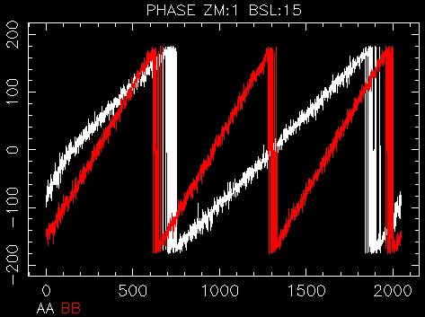
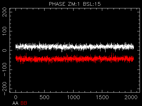
Once the majority of the delay error has been corrected for, the whole continuum band needs to be used for a second delay calibration:
cacor > calband f f | ||
caobs > corr dcal |
Pay attention to the value of delavg at this step to ensure that it is sufficiently low.
There are only a handful of channels to work with in the continuum bands in this mode!
|
|
|
| ||
|
Continuum band phase variations before delay calibration. This is the continuum band corresponding to the zoom band shown in Figure 3.9. It is clear (especially for the A polarization) that before any delay calibration, the average phases within each 64MHz continuum channel are not useful to determine a delay solution. |
Continuum band phase variations after zoom-band delay calibration. After performing delay calibration on the zoom bands, the phases have been largely flattened. The delays determined across a 64MHz frequency range are not sufficient to fully calibrate the continuum band, but they are sufficient to allow a refined delay calibration over the full continuum frequency range. |
Continuum band phase variations after final delay calibration. After performing a further delay calibration on the continuum bands, an excellent solution has now been obtained. This is apparent from the flatness of the phases across the full frequency range. |
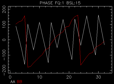
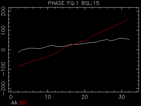
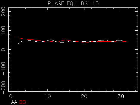
If observing at mm wavelengths, the antenna pointing should be checked and corrected before phase and amplitude calibration. A pointing scan has six separate pointings: first on the nominal on-source position, followed by four pointings at the nominal half-power points (+/- Az, +/- El), then a pointing back on the on-source position. A separate task, catag, calculates the pointing offets and feeds them back to the system to be implemented.
Check the pointing [1] page in MoniCA to check that the appropriate catag parameters are set:
User Antenna Maskshould include all antennas that need to be used for pointing.User IF Maskshould be set to include IFs that are required. 1234 uses all 4 IFs. 12 uses the two polarisations in the first frequency. 34 uses both polarisations in the second frequency. The setting 1234 can only be used if the frequenciesf1andf2satisfy .Integration Cyclesdefines the number of cycles spent on each step of the pointing solution. This will usually be set to 2 or 3.
Modifying these parameters is done in caobs
caobs > set point_a a1[a2
...a6] | defines antennas to be included in pointing calculations | |
caobs > set point_a 12345 | would use all antennas except CA06 |
Note: Pointing using the selfcal algorithm (default mode) requires 4
or more antennas to calculate gains. If using 3 or fewer antennas, holography mode is needed.
To enable holography, set the Integration Cycles to the negative (e.g. -2) value.
caobs > set point_if if1[if2...
if4] | defines IFs to be included in pointing calculations; | |
caobs > set point_if 1234 | would use both frequencies, both polarisations. |
(Note: If the two frequencies are different by more than 15%, the system will not let you use the second frequency. This is because the beam size is sufficiently different that problems can arise - think about the situation of a 5 and 10 GHz frequency pair. The half-power point at 5 GHz is the first null at 10 GHz.)
caobs > set point_p # | where # is the number of cycles spent on each pointing step. # is usually 2 or 3. If using holography mode, this should be -2 or -3. |
After these parameters have been set, ensure that your schedule file has a pointing scan set up.
This scan will need to have “Scan Type” set to “Point” and
the “Pointing” parameter set to “Update”.
To start the pointing scan, you must use the “start” command in caobs
(“track” will simply track the on-source position):
caobs > start # | where # is the scan number of the pointing scan. |
Watch the amplitudes in vis to check progress. You should see the amplitudes drop to approximately half the amplitude of the nominal centre position. The difference between the plus and minus pointings give an indication of the error in the pointing.
After the pointing scan has finished, check the errors that are found in the MoniCA pointing page. If any of the “Last Az Correction” or “Last El Corrections” is greater than 10″, a second pointing should probably be considered.
For more information on offset pointing, see the Reference Pointing Guide.
Phase Calibration is somewhat “cosmetic”, however, it can be useful to set the phases to zero at the start of observations to help judge the phase stability. To set the phases to zero:
caobs > corr pcal | pcal calculates the required correction and
applies the correction that the pcal offsets. |
(Early versions of the CABB software required an “a” switch at the
end of the acal command for the gains to actually be applied.
They are now applied automatically by the pcal command. Any switch other than an
a will result in the phase corrections not being applied.)
Once the delays have been set and pointing checked (for mm observations), the antenna gains need to be set. To set the gains:
caobs > corr acal [#1 #2] | acal calculates the required correction.
#1 and #2 are the fluxes of the calibrator
at the first and second frequencies respectively. |
(Early versions of the CABB software required an “a” switch at the
end of the acal command for the gains to actually be applied.
They are now applied automatically by the acal command. Any switch other than an
a will result in the gain corrections not being applied.)
If using PKS1934-638 or PKS0823-500,
the flux densities are known by caobs and do not have to be entered, i.e.
caobs > corr acal |
Gain settings are used for calculating Tsys. This can be recalculated off-line, but some care needs to be taken.
The Tsys values should be checked in the cacor GUI.
Any outlier readings should be checked.
At this point, the array should be set up and ready for observing. Check that all the products in vis look correct and that the Tsys values (in cacor) are appropriate. If there are any problems, check the Troubleshooting section Section 3.5.6 or get help.
When you have concluded setting up for observations and are prepared to begin observing, it is good practice to close the data file produced by the correlator so that the data produced during the setup process is not confused with useful calibrator and target data.
caobs> stop | ||
caobs> corr closefile | Closes the data file being written by the correlator in preparation for science observations. |
Once setup is complete, science observations can begin. Observations need to include calibration data, including data for flux density, bandpass, polarisation and gain calibration.
It is important that sufficient calibration data is taken to characterise the array. This means taking flux density and bandpass calibration data for all observations, and leakage calibration data for polarisation observations.
This does not have to be done at the start of the observation, but should be done at some point during the observing session. If appropriate calibration sources are not above the horizon during the observing session, contact the scheduler (Jamie Stevens) to discuss options.
For cm, 15mm and 7mm observations, PKS1934-638 is the
appropriate flux calibrator and can also usually be used as a bandpass
calibrator (although spectral line observations at 15mm or 7mm will ordinarily require a stronger source).
For 3mm observations, a planet is needed for flux calibration, and a
source with large flux density (e.g. PKS1921-293 or PKS1253-055)
is required to calibrate the bandpass.
Bandpass calibrators should ideally be observed at high elevation (above 40 degrees) if possible. This is especially important for excellent polarization calibration.
Once observing, the telescope will (mostly) look after itself.
The Fire and Primary Monitoring (PMon) systems monitor a number of critical telescope systems (e.g. power, cryogenics). Critical problems will trigger alarms which are distributed to site staff.
Observers need to monitor their own observations to ensure data quality. During observing, vis and spd should be checked semi-regularly to ensure that the data “looks ok”. In particular the observer should check that while on the calibrator: delays are close to zero, phases are flat(ish) and amplitudes remain constant. (There are a number of modes where some of these checks may be inappropriate, however, get help if it isn't obvious why these are not the case.)
The program assistance will often indicate that there is a problem with the system. Many of the error messages can be ignored if they are not relevant to the observations, however any unexpected errors should be followed up.
The MoniCA task displays monitor point information from antennas and other places.
The anemometer at the observatory measures local wind speeds every 2.5 sec. There are two (independent) systems that stow the array in the face of high winds:
xbones stows the array if the average wind speed for a 10 sec period is above 40km/hr
the PMon rack takes control of the array and stows if it detects a wind speed above 50 km/hr
Observers should respect this and not restart observing until the wind speeds have died down. In fact, if PMon has issued the stow you will have to wait 15 minutes until after the stow condition is no longer present before the antenna will be allowed to drive again.
In addition to high winds, electrical storms present a real danger to the ATCA. Storms and lightning strikes within a 56 km radius of the array are closely monitored. Threat levels (from 0 - no threat, to 4 - high threat) are assigned based on the number of approaching lightning strikes and those within 9 km of the array. When the threat level reaches 3, the back up generators are turned on. At a threat level of 4, xbones stows the array.
On very hot days (above 40°C), especially with a strong wind, the cryogenic compressors can become overwhelmed. In order to protect the receivers, if the ambient temperature in the internal system of the scroll compressors on the antennas (mm systems) reaches 91°C, xbones stows the array and turns the antennas to shadow the compressors from the wind.
Weather monitors (for wind, storms and heat) can be accessed in MoniCA. Alternately, the ATCA Weather Station also provides information about the weather.
If observing in the ATCA control building, you may hear alarms when certain problems occur. If you are observing remotely, you may ignore this section.
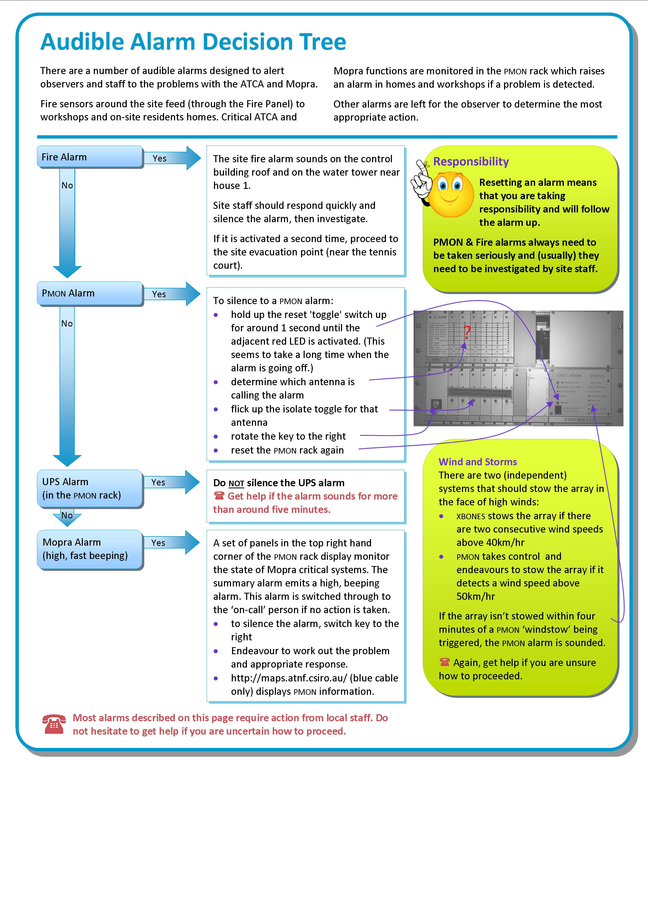
The first action in the face of an observing problem should always be to wait for at least a minute. (There are obvious exceptions to this rule, e.g. fires and similar catastrophic events that require quick action.) If waiting doesn't fix the problem, stop, restart and wait for at least another minute.
The following flowcharts provide details on how to recover from some of the most common observing problems. They explain what to do in the case of No Correlation (or funny correlation), Antenna(s) not 'on source', VNC Problems, and Rebooting a CABB block.
If you are unable to fix or diagnose your problem after following the flowchart you should call your Duty Astronomer. Sometimes you may be able to diagnose your problem but not be qualified to execute the required fix and in this case you should also call your Duty Astronomer. This may be the case if you need to reboot a CABB block, for example.
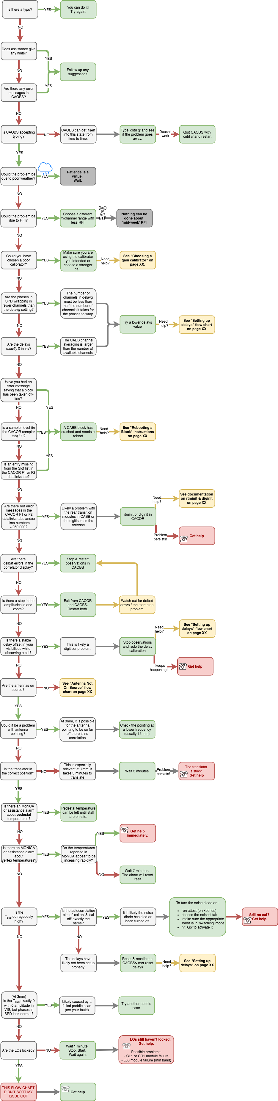
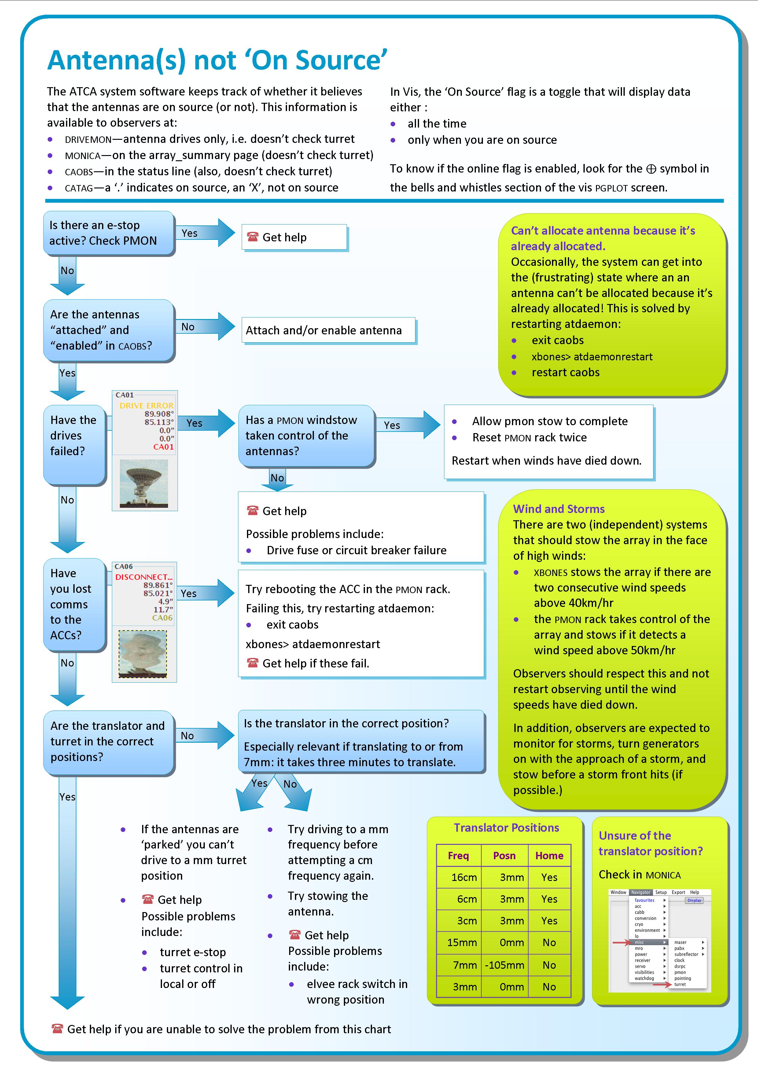
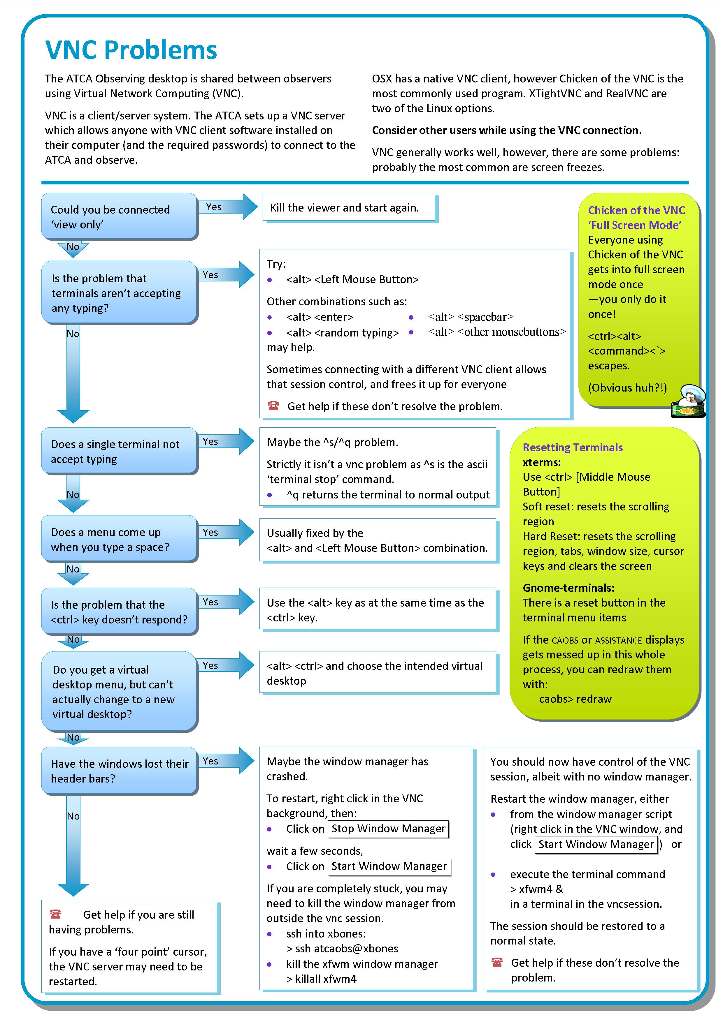
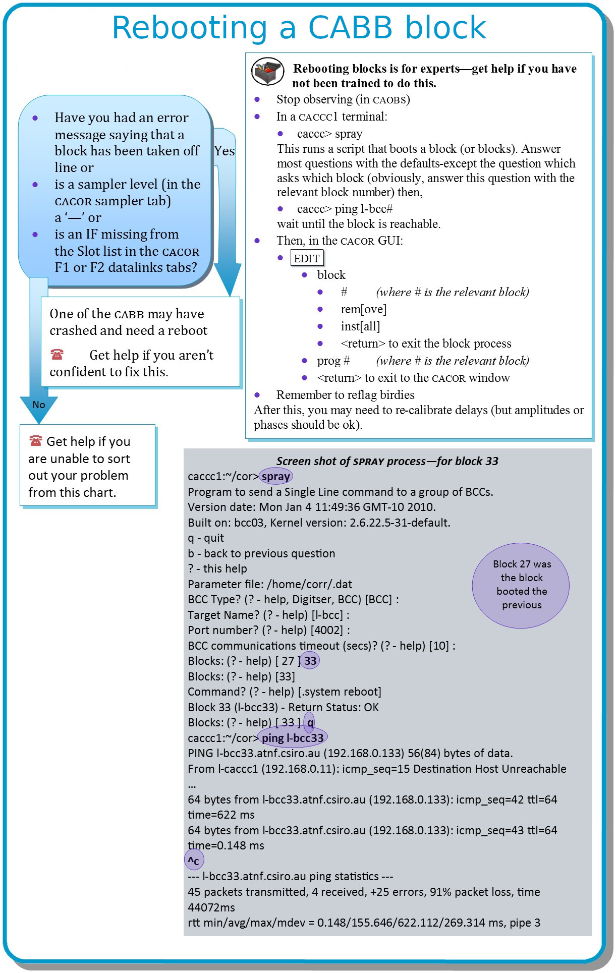
We realise that observers are busy people who cannot always be in front of their observing computer for the entire duration of their experiment. The observatory can be operated in “unattended” mode when it is convenient to do so. This section describes how best to observe in this way, and what is expected from you during your experiment.
When we talk about “unattended observing”, we mean any period during your experiment where you are not immediately aware of the state of the telescope. You may be any distance away from your observing computer, or asleep, or otherwise engaged in another activity, but you are listed as the “observer in charge” on the ATCA Portal.
The observatory does not require you to be responsible for the safety of the telescope equipment or of personnel. We have sophisticated systems and procedures which should handle any unsafe situation that might arise during a normal observation. For example, the automated systems will turn on the generators when a storm is approaching, and turn them off when it passes. It will also automatically handle stowing in periods of high wind, or when there is a high chance of lightning strike.
We do however expect that you are solely responsible for monitoring the quality of your data, and we do expect to be able to contact you via the phone number you supplied when you registered as the observer in charge. You should consider how often you need to check your data quality, given how much time you could lose if something goes wrong.
For example, if an antenna stops tracking due to a drive fault, you may call the duty astronomer and have them call the on-call person to remedy the situation; it might take only 10 minutes to rectify the problem if you were immediately aware of the fault. If you were asleep at the time of the fault however, you may lose a lot more than 10 minutes, and you would be ineligible to be compensated for that time. We recommend that even while sleeping through an observation, a periodic check is made every couple of hours.
We have developed several systems to proactively reach out to observers when something goes wrong that might need urgent action. This section describes the unattended observing alarm notification system available for the ATCA.
Whenever assistance detects a problem with the telescope hardware, or with the visibilities, it will make an audible alert - a bell sound - every 10 seconds while the fault is still present and not ignored. If you are sleeping, we recommend ensuring that you have the volume up loud enough for this bell so that it will wake you if necessary.
The MoniCA client has something called the “alarm manager”, which monitors many of the critical telescope systems. If a problem is found, it will start making sounds which approximate a robot saying “ATTENTION”. Again, we recommend that this be set up whenever you are within earshot of the computer, but are not paying attention to it.
The same alarms that will be displayed in the MoniCA alarm manager will also be turned into tweets on the ATCA Twitter feed. This should allow you to be a long way from your observing computer and still be alerted to problems with the telescope. Whenever an alarm is generated by MoniCA, or an alarm status goes away, a message is posted to the Twitter feed describing the problem.
A couple of example tweets are shown in Figure 3.14. Each tweet starts
with the UTC date and time that the alarm state changed. The date is listed as year-month-day, but
where the century part is omitted, to save characters. All alarms are given the hashtag
#ALARM; this may currently seem redundant, but this Twitter feed will likely be
expanded to include problems that do not generate MoniCA alarm states.
If an alarm has been triggered, then the next part of the tweet will be a hashtag describing how
important the alarm is. An #INFORMATION alarm simply presents a condition report,
but likely does not require any action. #MINOR alarms can be ignored until
it is convenient, where you should probably investigate #MAJOR and
#SEVERE alarms as quickly as possible.
If an alarm state has gone away, there will be no severity hashtag.
The rest of the tweet is then some guidance text about which system has caused the alarm. The guidance text is not designed to help you respond to or correct the problem; training on how to deal with problems that arise with the ATCA is still required. Rather, the tweet is there to quickly alert you to the problem.
The Twitter feed is still under active development, to make it as useful for observers as possible. All feedback about your experiences with the Twitter feed is welcome, as are suggestions on ways in which it can be made more useful.
The alarm notification system is based around Twitter because of the variety of methods
available to receive tweets on mobile devices. The simplest way of course is to install the
official Twitter client on your mobile device, and subscribe to the
@jamie_atca_sss Twitter feed from your account. In that way, you can make
your mobile device respond in one of several ways to any alarm tweets.
If you'd rather not set up a Twitter account, you can use the free online web service IFTTT (if-this-then-that) to respond in a customisable way to tweets from the ATCA alarm system. You will need to sign up to IFTTT, and connect your Twitter account to their Twitter channel, but after that you may specify any number of ways to get notification of tweets from the alarm system. For example, there is a published recipe that takes an alarm tweet and sends you an SMS. But you could also make your smart lights at home turn red, or get a phone call (in certain regions only).
Here is a list of key contact numbers (if dailing from an internal line, add an additional 0 before the number):
Emergency Services (fire, police, ambulance): 000
Duty Astronomer: 02 6790 4077
Observer: 02 6790 4078
On-call Pager (Narrabri): 02 6790 4076 (ring, wait a few sec, then dial 2)
SOC Astronomer Desk: 02 9382 4482
SOC ATCA Observing Room: 02 9382 4548
Marsfield Reception: 02 9372 4222
Narrabri Reception: 02 6790 4000
| Revision History | ||
|---|---|---|
| Revision 1.5 | 2021 Oct 19 | jbs |
| Remove references to kaputar, after it was turned off in Sep 2021. Update links that were no longer correct. Correct description of how importmiriad works. Update the recommendation of how to acknowledge ATCA in publications. | ||
| Revision 1.4 | 2018 Jun 19 | jbs |
| Add a section about what choices are available for data reduction, including Miriad, CASA and wsclean. Update all web links to HTTPS. Fix some typos. Remove some superfluous information about the old correlator. Describe quickly how to keep Miriad up-to-date. Add nopcorr=32 to everything 4cm and above, and describe why we don't use that in the 3mm band. | ||
| Revision 1.3 | 2015 Nov 19 | jbs |
| Describe pgflag and how to use it as an automatic flagger, with examples. | ||
| Revision 1.2 | 2015 Oct 21 | jbs |
| Removed section on portable hard drives, and recognised that CABB has been around for a long time now. | ||
| Revision 1.1 | 2014 Mar 24 | jbs |
| Revised to bring it up to date, and more detail in the data reduction section. | ||
| Revision 1.0 | 2014 Mar 20 | jbs |
| Initial Docbook revision | ||
There are several means for you to obtain a copy of your data once you have finished your observations. The following subsections will describe these methods in detail.
You are requested to make a copy of your data as soon as possible after the observations.
You can copy your data to your laptop from the Marsfield SOC. When your laptop is plugged in to a pink cable, you will have to use an SSH tunnel through venice to access the area on cetus where your data resides.
To set up the SSH tunnel, type the following in a terminal on your computer:
$ ssh -L 2222:cetus:22 usr123@venice.atnf.csiro.au
This makes all traffic directed at port 2222 on your computer get transported through venice to cetus via the usual SSH/SCP port of 22. This tunnel will exist as long as you remain logged into venice in this terminal. Thus to copy your data across, type the following in another terminal:
$ scp -P 2222 “usr123@localhost:/DATA/NEWDATA_1/ATCA/archive/*.CX167” .
which would copy all project CX167 data, and where usr123 is
your ATNF username.
If you are a CSIRO staff member and can connect your laptop directly to the ATNF network via a blue cable, you may copy the data directly from cetus:
$ scp “usr123@cetus:/DATA/NEWDATA_1/ATCA/archive/*.CX167” .
Your CABB data will appear on the Australia Telescope Online Archive (ATOA) within a few days of your observations. Using the OPAL account you used to submit your successful proposal, you will have access to your data. Full instructions for how to use the archive interface are available on the website.
If you are unable to get your data from the ATOA as soon as you would like, then you may get it directly from the disk on cetus that buffers the data.
To do this, you must set up an SSH tunnel from your local machine to cetus via the ATNF gateway machine venice. This can be set up with the command:
$ ssh -L 2222:cetus:22 usr123@venice.atnf.csiro.au
where usr123 is your ATNF username. This will log you into
venice and set up the SSH tunnel, which will remain until you
log out. To copy data from cetus
you should go to another terminal and do something like:
$ scp -P 2222 “usr123@localhost:/DATA/NEWDATA_1/ATCA/archive/*.CX167” .
After your observations, please provide us with feedback by completing the online Observer's Questionnaire. The feedback you give provides us with a way of measuring the success or failure of Compact Array operations, and allows us to identify areas that need attention.
If you can't find the information you require in this Users Guide and would like to ask our expert users how to do something, please visit the ATCA Forum website.You can also start or participate in conversations about your experiences with the ATCA.
There are now several software packages that are capable of reducing CABB data. For the purposes of calibration, the Miriad software package is still probably the best choice. It is possible though to do a full reduction without really using Miriad, if you prefer to use the CASA package. Below is a high-level comparison of what each package is capable of doing, and this may help you decide on how to proceed.
Only Miriad can read in raw CABB RPFITS files, with the atlod task. However, CASA can use its importmiriad task to take the output of atlod and convert it into the more commonly-used MeasurementSet (MS) format.
Both packages are capable of flagging CABB data, but generally speaking, the Miriad routines (such as uvflag, blflag and pgflag) are easier to drive, and give excellent results.
Both packages can do a full calibration of the data, including flux density calibration (the latest models for 1934-638 are in CASA), and polarisation calibration. The only significant difference is that CASA gives you much more control about where different effects are considered in the calibration tables; both will give excellent calibration however.
Imaging is where the Miriad and CASA packages differ greatly. Miriad allows you to make images over wide bandwidths, and does a good job of making spectral cubes as well. It also handles making mosaicked images, but lacks the ability to do mosaicking over a wide bandwidth.
To do that properly, you will need to turn to CASA, which is also able to handle doing multiscale cleaning, and does uv-based cleaning instead of Miriad's image-based cleaning.
For a simpler but more capable imager, you may also want to consider using wsclean, which supports most of what CASA does, but is very easy to drive.
This section will describe how to get started on reducing CABB data using the Miriad software suite. More information can be found in the Miriad manual. The manual's cookbook should be read by all users before starting their first data reduction. This section will summarise how reduction differs for CABB data, and give a reasonable guide on how to do a simple continuum reduction. The Miriad manual has been updated to incorporate information on CABB data reduction.
Miriad development is mostly static, but code to fix bugs may be introduced at any time. It is therefore important that before beginning your data reduction you obtain the very latest Miriad distribution.
To get the latest Miriad distribution, please follow the instructions in the install guide. Once you have it installed on your computer, it is easy to keep up-to-date. If you installed the binary version of Miriad (which is highly recommended), you can receive updates by running
$ mirsync -u usr123
where usr123
should be replaced with your ATNF UNIX user name. If you installed from source,
then you can use the mirimport command to get updates, after which you will
need to recompile Miriad.
It is also important to report any problems you may have with your reduction
to the Miriad maintenance team so that any issues can be resolved. If
you experience any problems, please use the mirbug routine, or send an
email describing your problem to <miriad@atnf.csiro.au>. If you don't
think your problem is related to a bug, but you need advice on how best to
proceed with your reduction, please ask for help using the
ATCA Forum.
ATCA and ATNF staff routinely check
the forum and answer questions from the community, making the forum a good
place to start to look for answers as well.
To load CABB data, you will use the atlod task. This section discusses how to use this command most effectively.
For CABB data, a number of channels are affected
by self-generated interference from the 640 MHz CABB clock, and the
birdie option flags these channels during load. It also flags out
4.9% of channels on each band edge (which works out to be 100 channels for CABB's
2049 channel spectra) and, for 20/13cm data taken before 2010-Aug-17, the unusable parts of the spectrum in
the old, separate 20cm and 13cm bands. These unusable parts are due to the fact that these
receivers did not respond to all frequencies across the 2 GHz bandwidth of
CABB. This option still works for pre-CABB data as expected.
If you wish to change the number of edge channels that are flagged by the birdie
option, use the edge parameter in atlod. By default it is
set to 9.8 (per cent), which works out to 200 channels for a 2049 channel spectrum. These flagged
channels are split evenly to the top and bottom of the spectrum, so if you wanted to flag only 32
channels on each band edge for example, you should specify
edge=3.1.
The rfiflag option can be used now to automatically flag out
frequency bands that are known to be heavily affected by RFI.
This option is most useful in the 16cm band, where the ATCA
receivers are routinely affected by strong RFI. It is completely safe to use at
any band however, and should be included in the default list of options when you
use atlod. The file it uses to determine the flagging it performs can be
customised to include extra flagging (or less flagging) if so desired. By default,
this file (called rfiflag.txt) can be found in the directory
cat in the Miriad tree.
To customise it, copy it to your reduction
directory, insert or remove more frequency ranges to flag, and then load your
data with atlod.
Note that the
rfiflag option will have no effect if the birdie option
is not also specified.
Another useful atlod option is xycorr. This corrects the
measured XY phase of the ATCA, and can be safely included at all bands for
CABB data.
By default, CABB records the autocorrelations from each of the antenna that
are being used, which may not be useful if all you are interested in is the
cross-correlations required to make an image. Having the autocorrelations
present during the reduction does no harm to any of the Miriad routines,
but may become confusing and/or annoying when trying to examine the data. You
can make atlod discard these data by using the noauto option.
The other atlod options are usually band-dependent. Examples of atlod use are given below for all ATCA bands.
- 16cm band
Task:   atlod
in       = *.C007
out      = c007.uv
ifsel    = 1
restfreq =
options  = birdie,xycorr,rfiflag,noauto
nfiles   =
nscans   =
nopcorr  =
edge     =
For this band, if you used identical centre frequencies in both IFs, you need only extract one of them as both IFs will contain identical data, and keeping both may lead to confusion later on.
- 4cm band
Task:   atlod
in       = *.C007
out      = c007.uv
ifsel    =
restfreq =
options  = birdie,xycorr,rfiflag,noauto,opcorr
nfiles   =
nscans   =
nopcorr  = 32
edge     =
If you chose to use the same centre frequency for both IFs then you should extract only 1 IF using the
ifselparameter as described above. As the frequency gets higher, the need to correct for atmospheric opacity increases; we recommend correcting for opacity in 32 separate frequency bins across the band (which is the maximum number of bins to use).- 15mm & 7mm bands
Task:   atlod
in       = *.C007
out      = c007.uv
ifsel    =
restfreq =
options  = birdie,xycorr,rfiflag,opcorr,noauto
nfiles   =
nscans   =
nopcorr  = 32
edge     =
- 3mm band
Task:   atlod
in       = *.C007
out      = c007.uv
ifsel    =
restfreq =
options  = birdie,xycorr,rfiflag,noauto
nfiles   =
nscans   =
nopcorr  =
edge     =
In the 3mm band, sky temperature (and thus opacity) is determined by the use of the paddle scan, so there is no need to include opacity corrections in the loading process.
For higher frequency data, the atfix routine may be required to apply corrections to the antenna positions and system temperature measurements.
During a baseline reconfiguration at the ATCA, staff perform a baseline calibration (to determine precisely where each antenna is with respect to each other) at 5 GHz and 17 GHz. During normal observing, the solution determined at 5 GHz is applied on-line, and is usually very good. However, for mm data, you may wish to use more precise antenna positions obtained from the 17 GHz baseline calibration. This may aid in phase referencing experiments.
The atfix routine can “fix” the positions of the ATCA antennas based on the solution file that is made available by the ATCA staff on the baseline solutions page. The high-frequency baseline solutions are not routinely computed for each reconfiguration, so if you'd like to have one, please contact ATCA staff with your request.
The task atfix is also highly recommended for the reduction of 3mm data.
During an observation at 3mm, the system temperature is determined using the
paddle during a so-called “paddle scan”. These scans are usually tens of
minutes apart, during which time the system temperature recorded by the
correlator does not change. To make Miriad interpolate the system
temperature between the paddle scans, use atfix with default parameters,
or with tsyscal=interpolate explictly set.
Task:   atfix
vis      = 3mm_data.uv
select   =
out      = 3mm_data_fixed.uv
dantpos  =
tsyscal  =
options  =
array    =
After loading the data into a Miriad dataset, it is usually most convenient to split this into many datasets, each containing an individual source at a single central frequency. This is done using the uvsplit task.
At its simplest, it can be run with only the vis parameter set to
the parent dataset, but it is also very easy to use the select parameter
here to discard data that was affected by antenna shadowing:
Task:   uvsplit
vis      = c007.uv
select   = -shadow(22.5)
options  =
maxwidth =
The select keyword can also be used to split out only certain sources,
or to effectively flag out certain antenna. Read about the select
keyword
in the Miriad manual.
There are two options that are useful here. Specify the
mosaic option if you are splitting a dataset that contains a mosaic
observation, and specify the clobber option if you want to overwrite
any previously split-out datasets in the current directory.
The maxwidth parameter is new to the CABB era, and allows you to
break up the 2 GHz CABB bandwidth into smaller chunks. This will be most useful
at lower frequencies where 2 GHz represents a large fractional bandwidth. At
such frequencies, calibration and imaging is far more challenging than at higher
frequencies. The bandwidth specified here should be specified in GHz. For example,
to mimic the maximum bandwidth available from the old correlator, you could
specify maxwidth=0.128 here. Recent experience shows
however that excellent calibration can be obtained using the entire 2 GHz band simultaneously, even
in the 16cm band. Splitting up the band at this point then is only recommended for those who have
an actual need to do so.
In most cases, if the birdie and rfiflag options are given
to atlod, the data will be mostly free from the most destructive RFI at this point. However,
you should always examine your data with the uvplt and uvspec tasks
to make sure.
Using uvplt, examining amplitude and phase versus time is a good way to
find time ranges that have been affected by RFI. Ensure that you specify
options=nofqav to prevent uvplt from averaging your data over
frequency before plotting. Any RFI present in your observations may
be restricted to only a few channels, and these channels can be identified
by using uvspec.
To flag this data, you can use the following tasks.
- uvflag
Use the
selectandlinekeywords to select the bad data and setflagval=flagto flag the data as bad. uvflag can be used to flag any set of bad data, but can be tediously repetitive.- blflag
This task can replicate many of the plots that uvplt generates, which may allow you to directly select the outliers representing bad data.
- pgflag
This task replaces the old tvflag task that no longer works on displays with more than an 8-bit colour depth. pgflag displays data as a channel-time waterfall plot and allows direct selection of ranges of bad data and flexible flagging options. It also includes an automatic flagging routine that uses the SumThreshold method that is available in the AOFlagger, and is highly recommended for use during continuum reductions.
One trap that you may find is that if you are observing at 3mm and some other band in the same run, and you elected to keep CA06 tracking for the 3mm observations, the data from CA06 will not automatically be flagged. This is because CA06 has almost all the systems required for 3mm observing (save for the electronics), and so the antenna really is “on source” according to the telescope. You should use uvflag to flag out CA06 data in this case.
Automatic flagging with pgflag can be very effective if it is done in the right way. It is most useful for continuum observations in any band, and for spectral line observations when the line is not detectable in a single integration. If your spectral line is bright enough to be detected in a single integration, then the flagging routine will likely identify it as RFI.
The pgflag task accepts a number of parameters that control the automatic flagging process. Craig Anderson identified, through trial and error, a recipe that works quite well for 16cm data; this recipe is described in an ATCA Forum post Craig started. We describe this recipe here as well, and we recommend this recipe for data in any band.
This flagging recipe uses the concept that the polarisation properties of interference are quite different to that of the signals we're interested in. For the most part, the radio sky is free of discrete sources of circular polarisation, and thus most measurements of Stokes V from our interferometer should be thermal noise only. This assumption holds over all frequencies as well. So if we see a large deviation from thermal noise in Stokes V, and this deviation is confined to a narrow range of frequencies, the most likely culprit is RFI. The first step of the flagging recipe then is to look for such signals in Stokes V and flag all the visibilities over the frequencies and times they are seen. To do this with pgflag:
$ pgflag stokes=i,q,u,v flagpar=8,5,5,3,6,3 "command=<b"
This flagging can be done on each individual source after it has been split out. Of course, because
the output of the interferometer should not vary for Stokes V regardless of the field being observed, you can
also flag a single IF all together. That is, you can take a dataset output by uvsplit
with options=nosource and flag it directly without further splitting it into
individual sources. You can also do the flagging before and after calibration. Indeed, you may
have success in doing an initial round of Stokes V flagging before trying to mfcal
the bandpass calibrator, and another round of flagging with the same command after
calibration.
As an illustration, Figure 4.1 and Figure 4.2 show what pgflag will display when told to show Stokes V from a dataset centred at 2100 MHz (a typical 16cm dataset) with fourteen scans on nine different sources, obtained in October 2015. Channel number is shown along the horizontal access, and as the 16cm band is presented to the correlator as a lower sideband, higher channel numbers correspond to lower frequencies. The time of the observation increases along the vertical axis towards the top of the image and the amplitude of each channel is represented as a grey scale which is outlined in purple toward the right of the image. Flagged regions are shown as completely black. Figure 4.1 shows a 60m baseline and Figure 4.2 shows a 4469m baseline. The only flagging done to this dataset is at the edges to remove the roll-offs, which removes 10.5% of the data on each baseline, and the data are uncalibrated. These two figures clearly show how much more sensitive short baselines are to RFI than long baselines.
Figure 4.1. A pgflag display showing Stokes V data on a short baseline in a 16cm dataset before flagging.
Figure 4.2. A pgflag display showing Stokes V data on a long baseline in a 16cm dataset before flagging.
After using pgflag as described above on the uncalibrated data, then bandpass calibrating and flagging with pgflag in the same way again, the data on the same baselines look like Figure 4.3 and Figure 4.4. Approximately 40% of the short baseline data is now flagged, and approximately 25% of the long baseline data.
Figure 4.3. A pgflag display showing Stokes V data on a short baseline in a 16cm dataset after flagging and bandpass calibration.
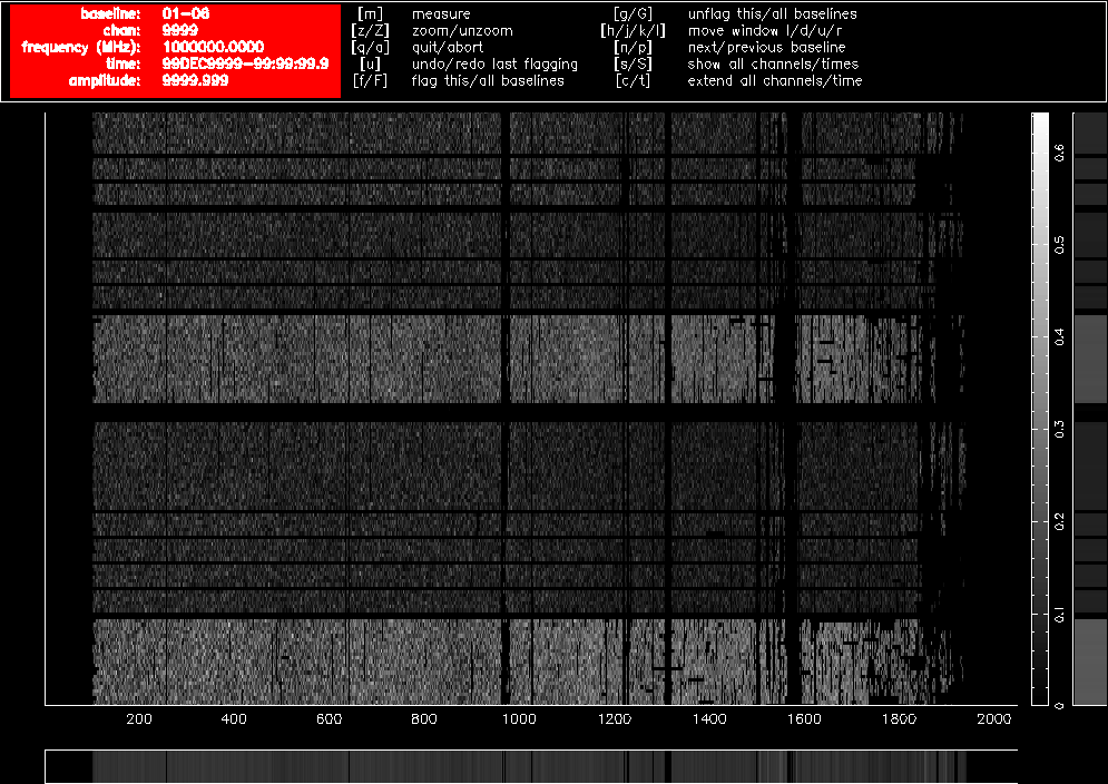
Figure 4.4. A pgflag display showing Stokes V data on a long baseline in a 16cm dataset after flagging and bandpass calibration.
As you can see, no obviously wrong signals can be identified in Stokes V after this process, but that does not necessarily mean that all RFI has been deleted from the data. Figure 4.5 and Figure 4.6 show Stokes Q on the same baselines as before, after the Stokes V flagging and bandpass calibration, and further RFI is obvious in those figures. We now flag using the linear-polarisation Stokes parameters Q and U.
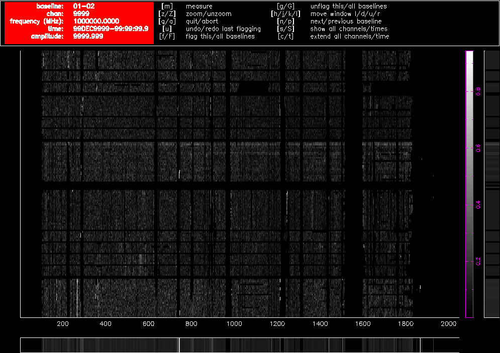
Figure 4.5. A pgflag display showing Stokes Q data on a short baseline in a 16cm dataset after flagging in Stokes V and bandpass calibration.

Figure 4.6. A pgflag display showing Stokes Q data on a long baseline in a 16cm dataset after flagging in Stokes V and bandpass calibration.
To do this we use pgflag as follows. First, flag Stokes Q:
$ pgflag stokes=i,v,u,q flagpar=8,2,2,3,6,3 "command=<b"
And then Stokes U:
$ pgflag stokes=i,v,q,u flagpar=8,2,2,3,6,3 "command=<b"
Again, these flagging commands can be done on each source individually, or on the dataset as a whole.
An example of how effective this flagging recipe can be is shown in Figure 4.7 and Figure 4.8. Using the calibration solutions derived from the flagged dataset, we can compare the 16cm spectrum of the calibrator 1953-325 before any flagging (Figure 4.7) to the spectrum after flagging (Figure 4.8). After the flagging process, only a small amount of RFI remains, and this is not likely to cause problems when measuring the continuum spectrum. On the shortest baselines, between 45-50% of the data has been flagged, but on the baselines to antenna 6 less than 30% of the data needed to be flagged. In terms of channels, 1625 of the channels have usable data out of the 2049 total channels, representing a spectral coverage loss of approximately 21%.
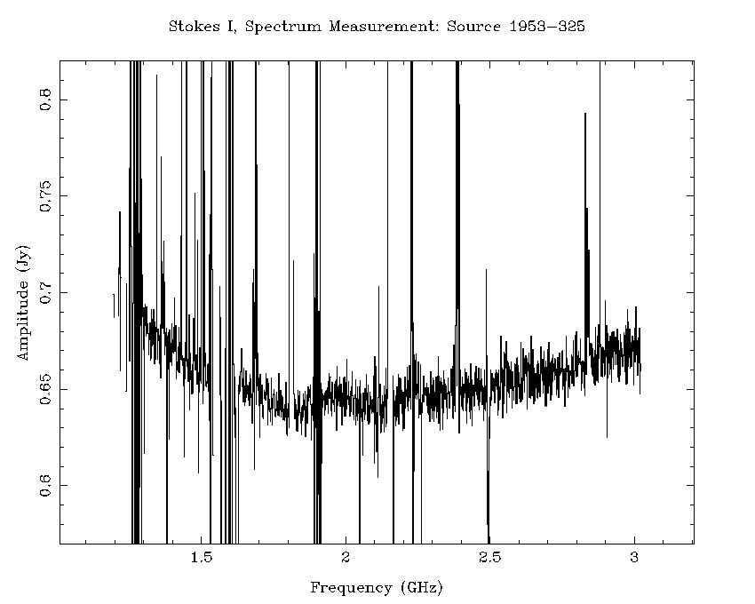
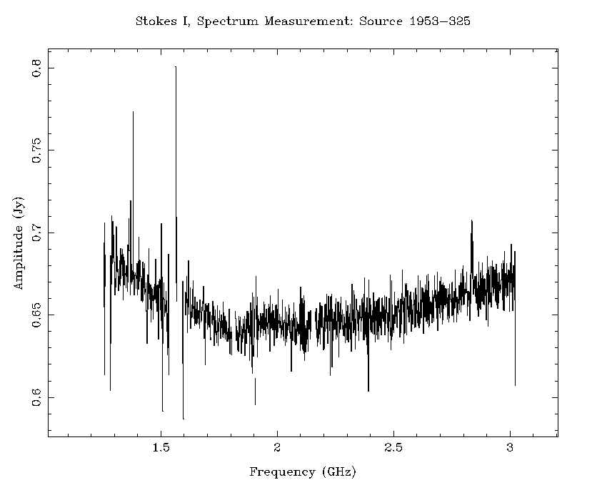
The calibration strategy for ATCA data has been refined for the CABB era, to ensure accurate calibration of wide bandwidths. This strategy also has the benefit of being applicable to the vast majority of ATCA data with little alteration. It is described best in the Miriad cookbook, but it will also be summarised here (although not explained in the same depth).
Calibration begins by determining the bandpass correction, using mfcal with
your bandpass calibrator. To prevent rapid gain variations from being entangled with your bandpass
solution, the interval parameter should be set to the cycle time (which is
usually 0.1 minutes). Since your bandpass calibrator should be very bright, such a short interval
should still have plenty of signal-to-noise. By default, mfcal uses
CA03 as the reference antenna, but if that antenna wasn't available during the observations,
ensure that you set refant to be an antenna that was available.
If you are reducing 3mm data, and CA02 was available, you should set it as the reference antenna. You should do this because it has the only noise diode in the array at 3mm, and setting it as the reference antenna may make it easier to do polarisation calibration.
| cm reduction | mm reduction |
|---|---|
Task: mfcal vis = 1934-638.2100/ line = stokes = edge = select = flux = refant = minants = interval = 0.1 options = tol = |
Task: mfcal vis = 1921-293.17000/ line = stokes = edge = select = flux = refant = minants = interval = 0.1 options = tol = |
Bandpass calibration in the cm bands (16 & 4) is usually done with the ATCA primary flux density calibrator 1934-638, as it has a large flux density at these frequencies. Since the flux density of 1934-638 is known as a function of frequency, the bandpass solution obtained in these bands is very good and takes into account how 1934-638 varies across the band. But if you use another calibrator for which Miriad doesn't have a flux density model, then the bandpass solution will be dependent on how that calibrator's flux density varies with frequency, which is a bad situation. You will need to correct for this, and how to do this correction will be described later on.
After bandpass calibration, the next step is to do some time-variable gain and polarisation calibration. If the bandpass calibrator is 1934-638, or if the bandpass calibrator has been observed several times during the run over a large range of parallactic angle, then you can use it for this step. Otherwise you should use the gain calibrator you observed.
| cm reduction | mm reduction |
|---|---|
Task: gpcal vis = 1934-638.2100/ select = line = flux = refant = minants = interval = 0.1 nfbin = 2 tol = xyphase = options = xyvary |
Task: gpcopy vis = 1921-293.17000 out = 2243-123.17000 mode = options = Task: gpcal vis = 2243-123.17000/ select = line = flux = refant = minants = interval = 0.1 nfbin = 2 tol = xyphase = options = xyvary,qusolve |
You should use an nfbin of at least 2 for all bands. This will
allow gpboot to correct any linear slope errors present in the
bandpass table. This also makes it unnecessary to use mfboot
unless your flux density calibrator is a planet. You should also increase the
interval parameter if the calibrator is not bright enough to
give enough signal-to-noise with 0.1 minutes of integration time.
If you used 1934-638 in the mfcal and gpcal steps, then you already have a flux calibrated dataset that can be used to fix the flux density scale on the other datasets.
You should now copy the solutions from the 1934-638 dataset to the gain calibrator dataset using gpcopy, and determine the time-variable gains with gpcal.
Task:   gpcopy
vis      = 1934-638.2100/
out      = 2243-123.2100/
mode     =
options  =

Task:   gpcal
vis      = 2243-123.2100/
select   =
line     =
flux     =
refant   =
minants  =
interval = 0.1
nfbin    = 2
tol      =
xyphase  =
options  = xyvary,qusolve
The gpcal step is likely to make the flux density scale on your gain calibrator slightly different to the true scale. To fix this you should use gpboot.
Task:   gpboot
vis      = 2243-123.2100/
cal      = 1934-638.2100/
select   =
You can now be confident that your gain calibrator is properly flux calibrated, and can now proceed to use it to analyse your science target.
At this point in the mm reduction, you need to do the flux density calibration. How this happens depends on whether you're using a planet as the flux density calibrator, or 1934-638. After copying the calibration tables from the calibrator used in the gpcal step to the flux density calibrator, you use gpcal followed by gpboot if you're using 1934-638, or mfboot for planets.
| 1934-638 flux calibrator | planetary calibrator |
|---|---|
Task: gpcopy vis = 2243-123.17000/ out = 1934-638.17000/ mode = options = Task: gpcal vis = 1934-638.17000/ select = line = flux = refant = minants = interval = 0.1 nfbin = 2 tol = xyphase = options = xyvary,qusolve,nopol Task: gpboot vis = 2243-123.17000/ cal = 1934-638.17000/ select = |
Task: gpcopy vis = 2243-123.33000/ out = uranus.33000/ mode = options = Task: mfboot vis = 2243-123.33000,uranus.33000/ line = select = source(uranus) flux = mode = clip = device = /xs options = |
Note the use of the nopol option for the options
parameter in gpcal, when 1934-638 is being used as the flux density calibrator.
This option tells gpcal that it should accept the leakage solution
obtained from the gain calibrator, which should be good since the gain calibrator is likely
to have much greater hour-angle coverage than the flux density calibrator.
In May 2016, Miriad's high-frequency flux density scale for 1934-638 was
changed to align the ATCA's scale to that of the VLA and the
absolute scale used by Planck. See Section 2.2.4
for details about this new scale. By default, after May 2016, Miriad
uses this new scale when setting the flux density of 1934-638 for frequencies above 11 GHz. The flux
densities measured from reductions using pre-May 2016 and post-May 2016
Miriad will therefore differ for observations above 11 GHz. If you would
like to keep using the pre-May 2016 flux density scale for 1934-638, you should use the
oldflux option that is available in the mfcal,
and gpcal commands.
At this point the gain calibrator will be reasonably well calibrated. If you are not especially concerned about flux density calibration accuracy, you can proceed to analyse your science target.
If you want to flux calibrate your data as well as possible, then you can use data from the other simultaneously observed band to improve your solution. Basically, the bandpass solution you made earlier assumed that the bandpass calibrator had a constant flux density with frequency (i.e. a flat-spectrum source). Because of this, the bandpass solution will likely be in error. Our gain solutions with two bins will have corrected this somewhat, but we can also try to emulate the situation in the cm band, and provide mfcal with a model of the flux density of the bandpass calibrator.
To do this, we copy the gain solutions from the gain calibrator back to the bandpass calibrator, recalibrate, and bootstrap the flux density scale.
Task:   gpcopy
vis      = 2243-123.17000/
out      = 1921-293.17000/
mode     =
options  =

Task:   gpcal
vis      = 1921-293.17000/
select   =
line     =
flux     =
refant   =
minants  =
interval = 0.1
nfbin    = 2
tol      =
xyphase  =
options  = xyvary,qusolve,nopol

Task:   gpboot
vis      = 1921-293.17000/
cal      = 2243-123.17000/
select   =
Note that these steps don't change regardless of the type of flux density calibrator you are using.
You should do the same calibration process with the other simultaneously observed band. At the end of the process you should have two bandpass calibrator datasets, each being flux density calibrated via the gain calibrator. You can now measure the flux density of the bandpass calibrator over the entire range of observed frequencies, using the uvfmeas task. The principle here is that even if the slope over a single band is wrong due to the incorrect bandpass calibration assumption, fitting a flux density model using two independently-calibrated bands should lower the uncertainties and provide a very good model of the actual flux density of the source.
Task:   uvfmeas
vis      = 1921-293.17000/,1921-293.19000/
select   =
line     =
stokes   = i
hann     =
offset   =
order    = 1
options  = plotvec,log,mfflux
yrange   =
device   = /xs
nxy      =
log      =
fitp     =
feval    =
The uvfmeas task does a linear least-squares fit to the log of the vector-averaged Stokes I flux density as a function of the log of the frequency. The plot it makes will show the averaged data in both bands, and the line of best fit (Figure 4.9). It will also output a string like:
MFCAL flux= 9.4126, 17.0,-0.3801
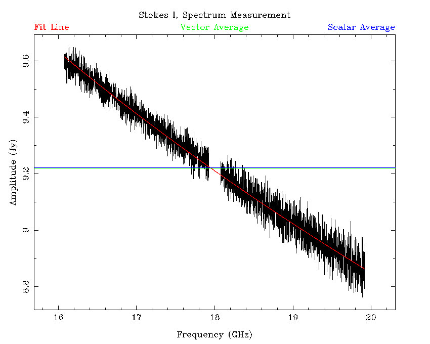
The string is usable as the flux in mfcal,
which will fit the bandpass solution while assuming the flux density model we just
determined. The image in Figure 4.9 is actually
the result of this two stage process, and you can see the excellent alignment
between the two bands, which are independently processed.
Once you have measured the flux density model for the bandpass calibrator, you must redo the calibration, but the bandpass calibrator becomes the flux density calibrator. The process is slightly different as well, and is summarised below.
Task:   mfcal
vis      = 1921-293.17000/
line     =
stokes   =
edge     =
select   =
flux     = 9.4126,17.0,-0.3801
refant   =
minants  =
interval = 0.1
options  =
tol      =

Task:   gpcopy
vis      = 1921-293.17000/
out      = 2243-123.17000/
mode     =
options  =

Task:   gpcal
vis      = 2243-123.17000/
select   =
line     =
flux     =
refant   =
minants  =
interval = 0.1
nfbin    = 2
tol      =
xyphase  =
options  = xyvary,qusolve

Task:   gpcopy
vis      = 2243-123.17000/
out      = 1921-293.17000/
mode     =
options  =

Task:   gpcal
vis      = 1921-293.17000/
select   =
line     =
flux     =
refant   =
minants  =
interval = 0.1
nfbin    = 2
tol      =
xyphase  =
options  = xyvary,qusolve,nopol

Task:   gpboot
vis      = 2243-123.17000/
cal      = 1921-293.17000/
select   =

Task:   mfboot
vis      = 2243-123.17000,1921-293.17000/
line     =
select   = source(1921-293)
flux     = 9.4126,17.0,-0.3801
mode     =
clip     =
device   = /xs
options  =
At this point both the bandpass and gain calibrator datasets will be very accurately flux density calibrated. Simulations suggest that this two-stage process can improve the flux density calibration accuracy to the 1% level for the bandpass calibrator, and to around the 3% level for any other calibrators referenced to it. Observations have confirmed this in the 15mm band, while for the 7mm band the flux calibration accuracy for an arbitrary gain calibrator is around 10%.
The calibration technique outlined above is robust and generally applicable, but may not work adequately for your data without alteration, and will almost certainly not work in an automated fashion. You should always be prepared to iterate between flagging and calibration, and you should use the visualisation tasks uvplt, uvspec and closure to check that the calibrator visibilities look as they should. You can also look at the calibration solutions directly using the gpplt task. Using uvfmeas to view the calibrators in both simultaneously-observed bands may also give you confidence that your calibration is good, or otherwise.
Imaging of CABB data can be performed in exactly the same way as pre-CABB data, however you may get better results with a slightly different method.
For high-frequency observations, where a bandwidth of 2 GHz does not represent a very large fraction of the sky frequency, then the imaging strategy used for pre-CABB data will most likely be adequate. For lower frequencies the multi-frequency strategies are more likely to produce good results. In particular, the use of the mfclean task should be considered. Read the excellent description of why mfclean is necessary in the Miriad cookbook to see if you will need to proceed with this strategy.
If you don't need mfclean then you should proceed with the usual invert, clean and restor method of creating an image, and combine this with selfcal or gpscal if appropriate. In this case, nothing should be different from pre-CABB reduction.
If you do need mfclean then the inputs to invert will need to be
slightly different as well. Firstly, both the mfs and sdb
options will need to be passed to invert. mfclean also requires
that the beam be three times the size of the region being cleaned, which can be quickly specified
in the latest version of Miriad in the imsize.
Task:   invert
vis      = obs.uv
map      = obs.map
beam     = obs.beam
imsize   = 3,3,beam
cell     =
offset   =
fwhm     =
sup      =
robust   = 0.5
line     =
ref      =
select   =
stokes   = i
options  = mfs,sdb
mode     =
slop     =
The first two options to the imsize parameter are usually the
number of pixels in the x and y direction respectively that the image will have. But when
you specify the beam option as the third argument to
imsize, the first two options are interpreted as multiples of the
FWHM of the primary beam at the central frequency of the image. In the example above, both the
dirty image and the synthesised beam image would cover 3 times the primary beam FWHM in each
direction. In earlier versions
of Miriad, both the imsize and
cell parameters would have needed to be determined manually and
explicitly set to do the same thing.
With the synthesised beam covering 3 times the primary beam FWHM, mfclean can be used to clean the entire primary beam.
Task:   mfclean
map      = obs.map
beam     = obs.beam
model    =
out      = obs.clean
gain     =
cutoff   =
niters   =
region   = percentage(33)
minpatch =
speed    =
mode     =
log      =
Here we are selecting the central third of the image (the primary beam
area) with the region keyword. This also satisfies the
mfclean requirement that a guard band be present around the
region being cleaned. The other parameters are very similar to those
of clean and should be set as usual to obtain good results.
After mfclean has run, restor should be used in the normal way to produce the cleaned image. selfcal can also be used in the usual fashion in this process.
Observers are requested to acknowledge the ATNF in any publications resulting from the use of the ATCA as follows:
The Australia Telescope Compact Array is part of the Australia Telescope National Facility (grid.421683.a) which is funded by the Australian Government for operation as a National Facility managed by CSIRO.
We also encourage an acknowledgement of our Indigenous community as follows:
We acknowledge the Gomeroi people as the traditional owners of the Observatory site.
The global research community is increasingly adopting persistent identifiers to improve how
resource use is cited and tracked. CSIRO has adopted the Global Research
Identifier Database (GRID) for its National Facilities and Collections, and the
ATNF acknowledgement statements now include these. The GRID code for all
ATNF telescopes is grid.421683.a. The use of a
persistent identifier ensures our facilities are consistently referenced and described
globally, and individual Digital Object Identifiers (DOIs) such as ORCIDs support the inclusion
of GRID codes.
Information about how to acknowledge other ATNF facilities is available on our website.
| Revision History | ||
|---|---|---|
| Revision 1.3 | 2021 Nov 12 | jbs |
| Fix incorrect description of how cain cal works. | ||
| Revision 1.2 | 2021 Oct 19 | jbs |
| Remove screen line for chat. Remove reference to caobs having a bell, which was removed after it was discovered it caused major problems with caobs in the latest Linux. Remove incorrect advice about the CA06 subreflector. Update advice on the use of the init command. Add a warning about starting a UTC schedule early. | ||
| Revision 1.1 | 2014 Apr 1 | jbs |
| Cleanup the text, remove some commands and add some new ones. | ||
| Revision 1.0 | 2014 Mar 20 | jbs |
| Initial Docbook revision | ||
caobs is the primary interface between the observer and the telescope. It coordinates the functions of the antennas and the correlator. It runs on xbones in a screen session, and is normally available from the main observing computer pericles and a VNC display from xbones.
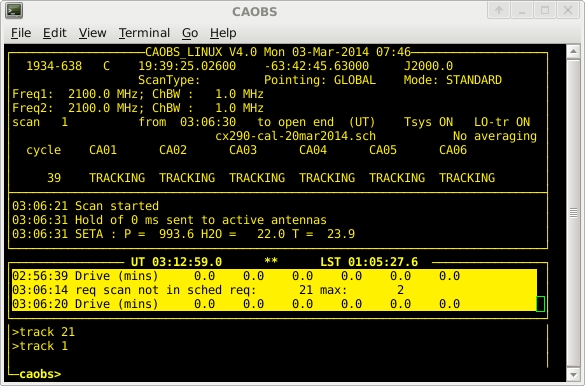
caobs will normally already be running before you start observing. If you cannot find caobs, try the following.
Check that cacor is running. (The cacor GUI is usually displayed in a separate VNC display from caccc1.) If it is not, start cacor as described in Appendix B.
Login to xbones and check for the normal screen session that is used to run caobs.
atcaobs@xbones:~$ screen -ls
The output from this command might look something like the following:
There are screens on:
        16310.catag	(06/03/14 15:26:40)	(Attached)
        5001.caobs	(05/03/14 15:07:17)	(Attached)
3 Sockets in /var/run/screen/S-atcaobs.
If you can see a screen session that is labelled with caobs, then you can reconnect to it:
atcaobs@xbones:~$ screen -x caobs
If you don't see a caobs screen session, then you can start one:
atcaobs@xbones:~$ screen -S caobs
Once connected to the caobs screen session, it should look something like Figure A.1. If it doesn't, then you can start caobs:
atcaobs@xbones:~$ caobs
Wait about one minute while caobs refers to its database and initialises.
Observers interact with caobs through a command line interface. Though there are many commands (see the Section A.1.1 section), there are only a handful that are used often.
-
caobs> set filefilename Loads the schedule file specified as the
filename. All ATCA schedule files have the extension.sch, but you don't need to supply this extension as part offilename.-
caobs> track# Tracks the source specified by scan
#of the schedule file forever (or until the source sets).-
caobs> stop Stops observing. This involves stopping the movement of the antennas, and stopping the correlator.
-
caobs> start#/n Starts observing scan
#of the schedule and proceeds to subsequent scans after each scan finishes. It will cycle through the entire schedulentimes before stopping, or until thestopcommand is given.-
caobs> corrcommand Sends the command
commandto the correlator GUI cacor, as if the command was entered into the GUI directly.-
caobs> stow Stows all the antennas that are attached and enabled in caobs.
Many of the commands that were part of the caobs command set
pre-CABB are now executed in the cacor processes.
Other commands are no longer appropriate. cacor commands
can be executed from within caobs by prefixing corr
in the caobs command. The following list
of caobs commands includes the cacor commands that
are often executed from within caobs.
-
attach ca0#|all Connect caobs either to antenna
#only, or all antennas. This command will fail for an antenna if the ACC in that antenna is dead or otherwise unavailable. Use this command to reconnect antennas that caobs reports as “OFF-LINE”.Related commands:
detach, disable, enable.-
cain calprescalecodecontinuous This command allows you to control of the noise diode on each of the attached antennas via the ACC. All of the three parameters are non-optional:
prescale: A prescale divider on the 1 MHz timeframe which controls the duration of the cal waveform pulses. Thisprescalenumber must be between 0 and 65535, but the actual prescale implemented by the hardware is this number plus 1.code: This is a further prescale by a factor of 2 to the power ofcode, wherecodeis between 1 and 8. This can be used to define pulses longer than what could be achieved within the 16-bit limits of the prescale divider by itself. It can also take some special values.continuous: Whether the waveform should be restarted at the start of each integration cycle (set to0), or only start it at the start at the first cycle and then continue to run freely at the specified frequency (set to1).
These numbers combine to give:
waveform cycle period = (
prescale+ 1) microsecondswaveform pulse duration = cycle period ÷ 2
As an example, the default ATCA waveform parameters are
prescale=31999,code=2, which gives a 128,000 μs cycle period. The ATCA cal waveform restarts at the beginning of each integration cycle, so the default is set by:cain cal 31999 2 0caobs will reset this parameter to the default values automatically at every change of observing project ID or at caobs restart.
-
cain cyclep|default Set cycle period to
pseconds, or to the default 10 seconds. For non-mosaicing observations, the cycle time can be set as low as 1.024 seconds, but when mosaicing the cycle time must be larger than or equal to 6 seconds, otherwise on-source flagging will not work.Note: The cycle time is generated in the ACC on each antenna, and this command will only be sent to the antennas that are attached at the time. If this command is given while some antennas are not attached, those antennas will have a different cycle time if they are later attached. Reissue this command to fix the inconsistency.
Related commands:
attach, detachcancelStops the current pattern (POINTing or mosaic).
Related commands:
point-
corr[elator]command Any cacor command can be executed from within caobs by prefixing the command with
corr[elator]. Commands that are often executed in caobs are documented here. See Appendix B for more complete information on cacor commands.-
corr[elator] acal [s1 s2] [a] Request that cacor perform an amplitude calibration.
s1ands2are flux density values for frequency 1 and frequency 2 respectively. If the source is PKS1934-638 or PKS0823-500, the flux density values are not required. For any other source, you can instruct cacor to calculate the likely flux density of the source (based on the expected system temperature) by usings1=0 ands2=0.The “
a” switch is now optional - the correlator will apply calibration by default. (To prevent the correlator from applying the corrections, replace “a” with any other letter).Related commands:
set referencecorr[elator] close[file]]Request that cacor close the current file. caobs must be stopped before executing this command.
cacor's display will show display “
FITS FILE: CLOSED” if this command succeeds. A new data file will be opened automatically when a scan is started, if a file is not already open.Related commands:
stopcorr[elator] dcal [a]Request that cacor perform the corrections required to make the phase flat across the band (i.e. caclulates geometric delay offsets).
The “
a” switch is now optional - the correlator will apply calibration by default. (To prevent the correlator from applying the corrections, replace “a” with any other letter).Related commands:
set referencecorr[elator] pcal [a]Request that cacor set the astronomical phases to zero.
The “
a” switch is now optional - the correlator will apply calibration by default. (To prevent the correlator from applying the corrections, replace “a” with any other letter).Related commands:
set reference
-
detach ca0#|allDisconnect caobs from either antenna
#or all antennas. No further commands will be sent to the disconnected antennas, until they are reattached.Related commands:
attach-
disable|enableparameter Disable or enable caobs or antenna-based functionality, depending on the
parameterspecified. Theseparameters are:disable|enable ca0#|allDisable or enable the drive machinery and turret rotator for either antenna CA0
#or all antennas. This will leave everything else as though it was observing.If an antenna is disabled via this command, caobs will show its status as “
DISABLED”.Related commands:
attach, detachdisable|enable correlatorDisable or enable correlation in cacor. If disabled, caobs will drive the antennas as normal, but the correlator will not output any data.
-
disable|enable lo Disable or enable the setting of the local oscillators and frequency conversion switches throughout the array. If disabled, the oscillators and switches stay in the state they were when this command was given, and do not change automatically with frequency changes in the schedule.
disable|enable turret [ca0#]Disable or enable rotation of the turret for antenna CA0
#if named, or the entire array if the argument is omitted. If disabled, the turret will not rotate automatically with frequency changes in the schedule.Note: Data will be flagged if the turret is in the wrong position, regardless of whether it is intentional.
-
disable|enable wvr [ca0#] Disable or enable the calibration of the water vapour radiometers on the named antenna, or on the entire array if the antenna is not specified. Calibration of the WVRs is done via a paddle on the mm receiver.
Note: Calibration of the WVR affects 7mm observations since the WVR paddle passes in front of the 7mm feed horn when it gets put in, or taken out.
Note: Calibration of the WVR is not actually required for effective use of the WVR data, and enabling the calibration is not recommended.
exitExit from caobs and return to the command line. You will need to stop the observations before issuing this command.
Note: You will need to exit caobs if you need to change cacor versions, or restart the atdaemon. If you are simply trying to exit the screen session that caobs is running in without affecting the operation of caobs, then you should use the key combination Ctrl+a d to detach from the session.
Related commands:
stopextendStop cycling through scans in a schedule file and continue the current scan indefinitely.
Related commands:
next, track, start-
focus {ca0#pos|default} Move the antenna subreflectors in order to focus the receivers. You can use this command in two different ways.
If you want to move the subreflector on a single antenna
#to the positionpos(in mm, from -24.0 to 24.0) then specify both the antenna and position.Example:
focus ca01 10If instead you wish to move the subreflectors on all the antennas to the positions recommended to focus each of them for the current observing frequency, simply give the argument
default.Example:
focus default
Note: Only attached and enabled antennas can be focussed.
initInitialise all caobs parameters to default values, and send initialisation commands to the antennas.
Treat this command with caution. It is very rarely useful outside of maintenance activities.
Related commands:
resetnextMove to the next entry in the schedule, i.e., move to the next scan. This command will cancel an
extendcommand and has no effect in mosaic mode.Related commands:
extend, start, trackpark [ca0#]Drives either the antenna CA0
#, or all antennas (if no argument is given to this command) to an azimuth of 90° and an elevation of 90°. Brakes are applied to the drives once this position has been reached. Observations must be stopped before this command will work. Only attached and enabled antennas will be parked.Note: This is the required position for antennas that are to be moved during a reconfigure. The antennas cannot be moved to this position if any of the mm receivers are on axis.
Related commands:
stop, stowpointnRuns a pointing scan on source
nin schedule. The actual definition of the scan in the schedule is irrelevant; only the source position and frequencies are used.Note: The program catag must be running for the pointing corrections to be calculated.
Related commands:
cancel, set point_pattern, set point_ifflag, set point_antennasppfixnLoads the pointing parameters determined by the pointing scan with the catag number
n. Any scans with pointing type “Offset” will now use this pointing solution, until a new pointing solution is made.ppglobalLoads the global pointing solution, as specified in the file
pparams.dat, into the ACCs. Any scans with pointing type “Offset” will now use the global pointing solution, until a new pointing solution is made.-
offset ca0#|alldazdel Force either antenna CA0
#or all antennas to track a position offset from that specified by the schedule file;dazanddelare the azimuth and elevation offsets in arcminutes. The offsets cease to apply at the next drive request (i.e., at the nextstartortrackcommand or when the next scan starts).-
reconfigparameter The
reconfigcommands are used when initialising and calibrating the array after a reconfiguration of the antennas. This is the only time when these commands should be used, and only by staff who have been trained in their use. Using these commands inappropriately could destroy your observations, and it might take several hours to recover.Each
parameteris described below.reconfig arraynameSelects new antenna array. The
namemust be identifiable with an entry in theconfigs.datfile. The positions of the antennas are changed to the appropriate station coordinates.reconfig bszeroSets the antenna offsets from the station coordinates to zero, by zeroing the file
station_errors.file. Before this command is executed, you should set the reference antenna to an antenna that hasn't moved; for most reconfigurations it should be set to CA06.Related commands:
set referencereconfig clearClears global delays, and delay and phase offsets.
reconfig ppinitResets global azimuth and elevation pointing offsets to defaults for the station posts used in this configuration.
redrawRefresh the screen. This command is useful for fixing the caobs display if it has become corrupted. If the display seems unresponsive, it might be because someone has issued a terminal stop command; in this situation
redrawwill not work, and you should try pressing Ctrl+q instead.reloadReload the schedule file.
reset ca0#|allResets the ACC for antenna
#, or all ACCs. Do not restart your observations until after the antenna image in the atdrivemon display has returned to normal.-
set|showparameter Set or show persistent caobs configuration parameters, or control antenna-based hardware. Not all
parameters can be used with bothsetandshow. Theparameters are:-
set|show atten ca0#a b Set the receiver module's attenuation levels for whichever receiver is currently being used (i.e. for the central frequency of the current scan). This includes the mm receivers, so this command can be used instead of the
set mmcommand. Unlike the CABB attenuators, the first attenuator setting (a) is applied to both “A” polarisations (A1 and A2) and the the second setting (b) is applied to both “B” polarisations (B1 and B2). Each attenuator step introduces (or removes) 1dB of attenuation to the signal path. There are 16 receiver attenuator steps (0-15).In general, this command should be executed while caobs is observing (i.e. the correlator is in the “GO” state).
With the installation of the 16cm and 4cm receivers on the array, all receivers now have controllable receiver attenuators.
Related commands:
set mmset|show avernAverage your data over
nintegration cycles in time. You must stop the scan before using this command. When observing large fields you should be careful not to average so much that you significantly distort your image (azimuthal smearing caused by time averaging increases linearly with distance from the phase centre). Refer to Appendix D of Killeen (1993) for details. The current averaging time is displayed on the caobs screen.Note: Time averaging can also be set in the schedule file.
It is not recommended that this parameter be used, since the data saved by cacor will be averaged by this amount and the unaveraged data cannot be recovered. It is better that you average the data later in data reduction if required.
Related commands:
cain cycle-
set|show band1_antennas## If you are attempting to use the ATCA's split-band observing capability, then you can use this command to specify which antennas should be allocated to each band. The set of antennas listed in
##will be allocated to the band specified by the IF1 central frequency, and all other antennas will be allocated to the IF2 band.Example: The command “
set band1_antennas 245” will allocate antennas CA02, CA04 and CA05 to IF1, while CA01, CA03 and CA06 will be allocated to IF2.This setting only has effect if the IF1 and IF2 central frequencies would put them in different bands.
set diode on|off|switchingControl the noise diodes on the antennas. For normal observations, this should be set to “
switching”. The “on” and “off” settings are only useful for maintenace.Note: The current state of the diodes cannot be shown in caobs, but is easily ascertainable by examining spd.
set|show el_limitnDefine the elevation limit to be
ndegrees. The hardware limit is 12°. You can use this command to skip sources in your schedule file below the specified elevation.Please reverse this setting at the end of your run so you don't surprise the next observer.
Related commands:
set rise_timeset|show filefilenameLoad the schedule file
filename, which must be in the directory/atca/schedon xbones. Thefilenamedoes not need to include the.schextension.The schedule filename will appear on the topmost section of the caobs screen.
set|show frequencyn cSet the central frequency of IF
n(1 or 2) to becMHz. All the normal frequency restrictions apply.set genset_on all|cb|ca0#Turn on all generators, or the generator for the control building only, or the generator for antenna CA0
#, respectively.This can be done without stopping observing, however it is important to monitor that the generator you commanded actually starts.
Only generators on attached antennas can be turned on.
Related commands:
attach, detach, set genset_off, show statusset genset_off all|cb|caO#Turn off all generators, or the generator for the control building only, or the generator for antenna CA0
#, respectively.This can be done without stopping observing, however it is important to monitor progress to make sure that the antenna or building you commanded returns to mains power successfully.
The power source will not automatically switch back to mains if a generator fails to start after it is commanded to start by the
genset_oncommand. If the generator fails to start, you will actually have to request that the generator be turned off with theset genset_offcommand.Related commands:
set genset_on, attach, detach, show statusset|show holdnThe
holdparameter is used to inhibit correlation only during those cycles affected by antenna movement. This command sets the hold period tontimes the automatically-determined hold increment for every cycle (normally 512ms), irrespective of antenna drives.To return to automatic hold calculation, given the command
set hold 0.show lengthDisplay the length of the current scan.
-
set|show mm ca0#a b Set the attenuation levels in the mm receiver. This command only works for the 15mm, 7mm and 3mm receivers. Unlike the CABB attenuators, the first attenuator setting (
a) is applied to both “A” polarisations (A1 and A2) and the second setting (b) is applied to both “B” polarisations (B1 and B2). Each attenuator step introduces (or removes) 1dB of attenuation to the signal path. There are 16 receiver attenuator steps (0-15).In general this command should be executed while caobs is observing (i.e. the correlator is in the “GO” state).
Related commands:
set attenshow modeDisplay the epoch currently being used by caobs.
show nameDisplay the name of the current source.
set|show paddle in|outOperates the room temperature paddle attached to the 3mm receiver. Normally, operation of the paddle is automatically done via the schedule file. This command should only be used for maintenance purposes.
set|show point_antennas##Defines which antennas catag will use to calculate pointing corrections.
Example:
set point_ant 234would allow pointing corrections to be calculated for antennas CA02, CA03 and CA04.Note: There appears to be a bug in catag such that if an antenna is added to the
point_antennasset, the first pointing scan done after this command is given will not compute corrections for the added antenna. You can simply redo the pointing scan to compute the corrections.Related commands:
point, set
		    point_pattern, set point_ifflag
set|show point_ifflag##Defines which IF channels catag will use to calculate pointing corrections. Pointing corrections are not made as a function of polarisation or frequency, so this parameter just allows you to average more data to get a higher signal-to-noise ratio and therefore a more accurate solution.
Example:
set point_if 12would make catag use polarisations A and B in IF1.At mm frequencies, this parameter should normally be set to
1234. If the IF1 frequency differs from the IF2 frequency by more than 30%, then the primary beam in one IF will be too different to the other IF to use them both simultaneously to calculate pointing corrections. In this case, catag will automatically change this setting to12.Related commands:
point, set
		    point_pattern, set point_antennas
set|show point_patternnSpecify the number of cycles (
n) caobs will direct the antennas to spend on each offset position during a pointing scan.If
nis a positive number, the “selfcal” pointing procedure is used, whereby all the antennas move to each offset point at the same time. There must be at least four antennas enabled for this mode of pointing to work.If
nis a negative number, holography mode pointing is performed. In this case, all the antennas but one (a reference antenna) move to the offset positions. After the first round of pointing is done, a new reference antenna is chosen, and the process is repeated; in this way the pointing corrections are calculated for all the antennas, but it takes twice as long as selfcal mode. Use this pointing procedure only if you have fewer than three antennas available.Note: The actual value of
nis usually set to2. catag only requires one integration at each offset point to do the pointing correction calculations, but two will increase the signal-to-noise-ratio. With CABB's bandwidth,nrarely needs to be set higher than2. In the past, a pointing correction used to fail if one antenna did not make it on source in time for at least one cycle at any particular offset position; caobs now ensures that this can no longer occur, by adding extra cycles when required to allow the antenna to get on source.Related commands:
point, set
		    point_ifflag, set point_antennas
set|show reference#Set the reference antenna to be CA0
#. This will communicate the change automatically to the correlator. Using this command in caobs is required for holography-type experiments, where one antenna does not participate in an offset pointing program, and during the reconfiguration process.set|show rise_timenIf a source is below the horizon when it is scheduled to be observed, caobs will wait for up to
nminutes for the source to rise. If the source will not be up in that time, the array skips this source and moves to the next source in the schedule file.Related commands:
set el_limitset scanlengthh:m:sIf you set the position to be observed using the
track 0command, you can set the length of the scan with this command.Related commands:
trackset sourcesourcenameIf you set the position to be observed using the
track 0command, you can modify the source name with this command.Related commands:
trackshow startDisplay when the current scan started, as UTC.
show statusDisplay general array information. Normally, the top panel of caobs will look as it does in Figure A.1. If you turn the generators on or off though, the top panel will be replaced with a warning about generator operation. To make caobs display the normal top panel again, use this command.
-
start [n[,k][-m][/l]]Commence automatic scheduled observations once you have used the “
set file” command to load your schedule file. The schedule file will then control the activity of the telescope.This command can be used in a number of different ways:
If you are running a schedule that has scan starting times defined as UTC datetimes, then simply issuing the “
start” command will start with the scan that should be currently running, and change scan as required.Note: With a UTC schedule, any arguments to the “
start” command will be ignored, and caobs will follow the schedule exactly as defined.If you are running a schedule that does not have absolute UTC scan start times, issuing the “
start“ command with no arguments will make caobs start with scan 1 and continue running the schedule file until there are no further scans.Note: This is equivalent to giving the command “
start 1/1”.If you wish to start the observation with a scan defined in the schedule file as scan number
n, then you can supply this scan numbernas the first argument.Example: “
start 2” will start observing on the second scan defined in the current schedule file, and continue observing until the end of the schedule file is reached.If you wish to start the observation with a scan defined in the schedule file as scan number
n, and continue until the scan defined as scan numbermis finished, then you can supply both thenand-arguments.mExample: “
start 2-8” will start observing on the second scan defined in the current schedule file, and continue observing until the end of the eighth scan is reached.If you want to begin observing with a scan on a position defined in a mosaic file, that is not the first source defined in the mosaic file, then you can include the optional
,argument, wherekkis the line in the schedule file (not including comment lines) that the source is defined on.Example: “
start 2,3” will start observing with the third position defined in the mosaic file that is referenced in the second scan of the schedule file. caobs will then continue observing until the end of the schedule file is reached.If you want to make caobs loop repeatedly over a set of scans, starting with the first defined scan and ending with the last defined scan before repeating the process, then you can use the optional
/argument, wherellis the number of times to loop over the scan range.Example: “
start 2/10” will start observing on the second scan defined in the current schedule file. When the last scan in the schedule is finished, caobs will continue observing starting with the first scan defined in the schedule file. After the last scan defined in the schedule is observed for the tenth time, caobs will stop observing.Example: “
start 2-8/10” will start observing on the second scan defined in the current schedule file. When the eighth scan in the schedule is finished, caobs will continue observing starting with the second scan defined in the schedule file. After the eighth scan defined in the schedule is observed for the tenth time, caobs will stop observing.Example: “
start 2,3/10” will start observing with the third position defined in the mosaic file that is referenced in the second scan of the schedule file. When the last scan in the schedule is finished, caobs will continue observing starting with the first scan defined in the schedule file. Subsequently, whenever the mosaic referenced in the second scan is observed, it will start at the first defined position. After the last scan defined in the schedule is observed for the tenth time, caobs will stop observing.
There are several caveats to using the “
start” command.If the source that is next in the schedule is below the elevation limit set by the “
set el_limit” caobs command, and the source will rise within the time defined by the “set rise_time” command, then caobs will move the antennas to intercept the source as it rises above the elevation limit. During this time, the correlator will be ready to run, but will not be producing data; you may see an error message in assistance stating that there is no recent data from the correlator.If the source won't rise within the rise time limit, then caobs will simply skip the source and continue to the next one in the schedule. If there are no sources in the schedule that are above the elevation limit, and won't rise within the rise time limit, then the behaviour of caobs may be strange; expect plenty of beeps.
If the source that caobs is tracking sets during the scan, caobs will move to the next source in the schedule, if possible.
If you command caobs to start a UTC schedule before the start time of the earliest scan, then it will prepare the correlator, but will not direct it to produce data, and the antennas will not move. Until the UTC of the first scan, you may see an error message in assistance stating that there is no recent data from the correlator.
WARNING: In this case, the correlator will NOT start until the start time of the scan you have started. Even if you stop the scan in caobs and start another, the correlator is waiting for the previous start time and cannot be interrupted. In other words, DO NOT START A UTC SCHEDULE BEFORE THE START TIME OF ITS EARLIEST SCAN.
Related commands:
stop, track, point, set rise_time, set el_limit, attach, detach, enable, disablestopStops the current scan. The antennas will stop moving and the correlator will stop producing data. Use the “
correlator closefile” command to close the data file. A stop command is always sent to all attached and enabled antennas, even if no scan is underway.Related commands:
start, track, corr closefilestow [ca0#]Drives either the antenna CA0
#, or all antennas (if no argument is given to this command) to an azimuth of 90° and an elevation of 85°. Brakes are applied to the drives once this position has been reached. Observations must be stopped before this command will work. Only attached and enabled antennas will be stowed.Note: This is the preferred position for idle antennas. This command should be given at the end of your observation if the next observer is not ready to begin, or if there is no observing scheduled to begin within 30 minutes of your observations ending. This is also the recommended position for antennas during periods of high wind or during storms.
Related commands:
stop, parktrack [n]Track the source described in scan
nof the current schedule file, until either astopcommand is issued or the source sets. Ifnis omitted, the first source in the schedule file will tracked.If
nis “0”, caobs will track a position using the current settings (usually from the previously-tracked source). The current caobs settings can be modified by a number ofsetcommands.Related commands:
start, stop, set source, set frequencywrap north|southSpecify the antenna azimuth wrap that should be used to track the next specified source. This command will only have an effect if caobs is stopped at the time, and if the next command given is “
start” or “track”. Anything else will cancel the request.You can demand the antenna wrap on a per-source basis in the schedule, using the “
Wrap” parameter (an advanced parameter) in the CABB web scheduler.Related commands:
start, track
| Revision History | ||
|---|---|---|
| Revision 1.4 | 2021 Oct 20 | jbs |
| Clarify how CABB calculates delay slopes. Fix imprecise language. Remove advice about not using 0823-500 for 64 MHz zoom calibration at 16cm. Add description of tvmedian. | ||
| Revision 1.3 | 2018 Jun 19 | jbs |
| Fix some typos, and change some recommendations about how to use certain commands. | ||
| Revision 1.2 | 2015 Oct 20 | jbs |
| Fix some typos | ||
| Revision 1.1 | 2014 Apr 13 | jbs |
| Cleanup the text, and update the command list for the currently used cacor versions | ||
| Revision 1.0 | 2014 Mar 20 | jbs |
| Initial Docbook revision | ||
The cacor program controls the correlator and correlator functions. It runs on caccc1 and is normally displayed on a VNC display.
cacor will normally already be running before you start observing. If it isn't, start it by typing:
caccc1:~> cacor
A display similar to that shown in Figure B.1 should now be visible on the caccc1 VNC screen.
If you restart cacor, then caobs will also need to be restarted afterwards. For instructions on how to do this, please consult Appendix A.
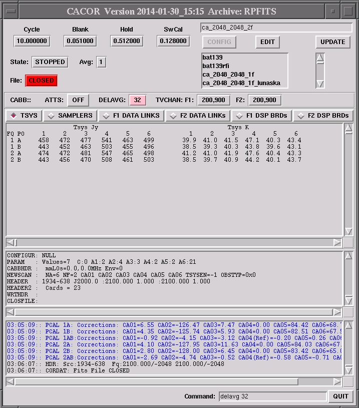
The cacor window has five panels:
Observers can interact with cacor through the text input box located at the bottom of the GUI, between the “Command:” label, and the “QUIT” button. We call this the “Command” entry box. The full list of commands that can be issued through this interface is below.
-
abphasen m Set the desired phase offset (in degrees) to insert between the A and B polarisations of each antenna, where
nis the desired offset in IF1, andmis the desired offset in IF2. The phase offset will not be inserted however until a “pcal” command is issued.The most useful purpose for this command is to switch between linear polarisation (for which
nandmare both 0) and circular polarisation, which requires a phase shift of ±90° between the linear feeds, depending on the sideband. This is most commonly used for VLBI experiments, which record circular polarisation.Example: The command “
abph -90 -90” will produce circular polarisation output from the tied array units, for USB frequencies.Related commands:
pcal, catie polacaln m[a-z]Tells the correlator that the average flux density of the source currently being observed is
nJy over thetvchannelsset in IF1, andmJy over thetvchannelsset in IF2. The correlator uses this information when calculating the system temperature that it writes into the RPFITS files.If the command is given with or without a trailing “
a” option, then the correlator will apply the calibration. If the trailing option is specified as any letter other than “a”, the correlator will display the corrections it would make, but will not apply them.Related commands:
dcal, pcal, tvchannels, reset acal, calband-
attfca0#n m Set the amount of CABB attenuation on IF1 (“
att1”) or IF2 (“att2”), for antenna CA0#, to bendB for polarisation A andmdB for polarisation B.The current CABB attenuator settings are shown in the “Sampler Levels” tab in the data panel.
There is an attenuator servoing command that will adjust the CABB attenuation automatically to equalise signal levels across antennas and polarisations. This command is “
attservo”.Related commands:
attservo, tattservoattservo [on|off]Attenuator servoing will make the correlator attempt to bring the sampler/GTP statistics into line with the target that was set with the “
tatts” command. It does this by adding or removing CABB attenuation on a per-antenna, per-polarisation, per-IF basis. It may take a relatively large number of cycles (more than 5) to accomplish this, and may not be able to precisely meet the target specified.Without arguments, this command returns the current state of the attenuator servoing mechanism (which can also be found in the status panel). To start/stop the servoing mechanism, issue this command with the “
on/off” argument respectively. It is important to check the resultant attenuation levels (shown on the "Sampler Levels" tab in the data panel) for potential problems during this process.Related commands:
tattservo, userms, usegtpcalband [n m]This command changes the IFs that the correlator uses to determine the delays, phases and amplitudes. The setting that you can make here depends on the cacor version, and the correlator configuration.
While observing with a configuration that provides the 2 GHz continuum IFs with 1 MHz resolution (eg. “
ca_2048_2048_2f”), these quantities should be calculated from the continuum IFs at all times. To ensure this,nandmshould both be set to “f” if the cacor version is not one designated for VLBI use, or “0” otherwise.If the frequency resolution of the 2 GHz continuum IFs is worse than 1 MHz (eg. “
cfb_64_32_2f_zm16”), or if the correlator configuration does not provide the 2 GHz continuum IFs (eg. “cfb64_vlbi”), then it may be necessary to use the zoom bands to compute and/or correct the delays and phases. In this case, bothnandmshould be set to “z” in non-VLBI cacor versions, orn=3(the first zoom IF) andm=4(the second zoom IF) otherwise.All the commands that affect the computation of delay, phase and amplitude (eg.
tvchannels, dcal, pcal, acal, delavg) will apply to the IF that is specified by this command.Note: When in a non-VLBI cacor version, the “
z” setting fornormcan only be used if the first specified zoom in that IF has a width of 1 (i.e. the zoom band is not a composite zoom). If this is not the case, the correlator will return an error message.Related commands:
acal, dcal, pcal, tvchannels, abphase, delavgcalfreq [f]Specify which IF (1 or 2) to use when manually correcting the delay with the “
doffset” command. Without arguments, this command will return the currently selected IF.Related commands:
calpol, doffsetcalpol [p]Specify the polarisation (a or b) to use when manually correcting the delay with the “
doffset” command. Without arguments, this command will return the currently selected polarisation.Related commands:
calfreq, doffsetcalrefant [#]Set the reference antenna for calibration purposes to be CA0
#. As with “refant”, this is usually best set to antenna 2, if it is included in the array. If this command is issued without arguments, it returns the current setting of this variable.Related commands:
refant, dcal, pcal[ca]tie [command[##]]The correlator can be take the signals from each of the ATCA antennas and combine them in real time to form a single output phased up towards a nominated phase centre: this is called the “tied array”, and is usually configured for VLBI observations. The “
catie” commands configure this tied array.The tied array commands can be prefixed with “
catie”, or, in a slight reversal of the usual minimum-match pattern recognition, it can be shortened to “tie”. When issued without an argument, cacor will return the current configuration of the tied array.The tied array commands and their optional arguments are described below. Each of the tied array commands take two optional arguments, which control each of the two IFs. It is not possible however to control one IF with these commands without simultaneously having to set the state of the other IF.
-
[ca]tie array [## ##] Tie the signals from antenna(s)
##into the tied array output, per IF.Example: The command “
tie array 123 245” ties the signals from CA01, CA02 and CA03 into the IF1 tied array output, and from CA02, CA04 and CA05 into the IF2 tied array output.-
[ca]tie pol [t t] Configures the tied array to either output directly the two linear polarisations (
t=l), or to combine the two linear polarisations together to output circular polarisations (t=c).Example: The command “
tie pol l c” would leave the linear pols as is for the tied array output of IF1, and form circular polarisations for the tied array output of IF2.Note: The “circular” polarisation setting here does not automatically form circular polarisations; it simply combines the two linear polarisations together with the current cross-polarisation phases. This command must be used together with the “
abphase” command to properly form circular polarisations.Related commands:
abphase-
[ca]tie gain [n n|auto] Sets the gain for the tied array output for each IF to be
n, where 0 <n≤ 1. This gain setting, combined with the GTP sampler statistics, is able to vary the amount of power fed into the DAS units.If all antennas are tied, and the GTP statistics are around 30, then a gain of 0.1 is recommended.
Example: The command “
tie gain 0.1 0.09” will set the tied array gains to 0.1 and 0.09 on IF1 and IF2 respectively.The gain can be set to change automatically by supplying the
autoargument instead of the IF gains. Automatic gain control can only be set to work for both IFs simultaneously; it cannot work for a single IF only.Related commands:
tattservo, attservo-
[ca]tie reset Resets the output from the tied array output module in the correlator. The configuration of the tied array outputs will not change.
-
-
cf [n m] The CABB system's primary frequency band corresponds exactly to the 4cm band, where 3904 MHz ≤ ν ≤ 11952 MHz; all other frequency bands are mixed into this range using front-end LOs. To select the two 2048 MHz intermediate frequency ranges (the CABB IFs), we use the CL1 LO modules, which can be tuned between 4928 MHz ≤ ν ≤ 10928 MHz.
This command either lists (if no arguments are supplied), or sets the CL1 frequency to
nMHz for IF1, andmMHz for IF2.You must set the CL1 frequency for both IFs when you issue this command. If one or both of the frequencies are out of the accepted range, the command will not work. cacor will output the new LO frequencies after this command is given.
Note: The IF frequencies are set by caobs, not cacor, so changes to the centre frequencies using this command will not be reflected in the output data file.
[no]czabsThis command enables (with “
czabs”) or disables (with “noczabs”) the correlator's auto-correction and online application of the zoom bandpasses. Since the zoom bands are digitally constructed, their bandpass shapes can be accurately determined during the observation, and corrected before being written out to the data file.Use this command to disable this behaviour, as it is enabled by default.
dcal [a-z]Tells the correlator to estimate the delay in each of the IFs set with the “
calband” command, using the data in the “tvchannels” range, boxcar averaged over “delavg” channels, for the previous “nncal” cycles, with respect to the reference antenna set by the “calrefant” command.If the command is given with or without a trailing “
a” option, then the correlator will apply a correction to compensate for the calculated delays. If the trailing option is specified as any letter other than “a”, the correlator will display the calculated delays, but will not apply them.Related commands:
acal, pcal, tvchannels, delavg, calband, nncal, reset delays, calrefantdelavg [n]To calculate the delay in any particular IF, cacor looks at the phase in each channel in the “
tvchannels” range and calculates the average line slope between each pair of phases as a function of frequency; this average slope is the delay.If the noise on the phase is high (due to low signal-to-noise ratio or poor weather, for example), or there is some strong unavoidable RFI in the “
tvchannels” range, then the average line slope may not accurately represent the real slope due to the delay.To reduce the noise, or to average out the effect of the RFI, you can use this command. This command tells cacor to first average together each
nchannels in the “tvchannels” range before calculating the average slope.Example: Suppose the “
tvchannels” are set to include channels 513 to 1537 (a total of 1025 channels). With a “delavg” of 1, the delay slope calculation would use 1025 points. If you set “delavg” to 4, then the delay slope calculation would use only 256 points, and each point would have a signal-to-noise ratio 2 times better than with “delavg”=1.This command is especially useful at higher frequencies, and is almost necessary in the 3mm band, due to the lower sensitivity of that receiver. It is also very useful when doing the delay calibration using a single 64 MHz zoom, since the bandwidth of each channel is greatly reduced.
Related commands:
tvchannels, dcal, calband[no]delscan ff offset,incrIf it isn't possible for some reason to have cacor automatically compute delay corrections, it is possible to use this command in order to manually determine the delay between each antenna and the reference.
This command makes cacor cycle through a range of delay offsets for IF
f, starting at -offsetns (compared to the current setting per antenna), and addingincrns of delay to each antenna at each subsequent cycle.By looking at the amplitudes at each cycle, it is then possible to determine which offset is closest to the systemic delay for each antenna. These offsets can be added into the correlator with the “
doffset” command.This command will continue to operate until the “
nodelscan” command is issued.Example: The command “
delscan f1 -40 4” will make cacor subtract 40ns of delay from each antenna (except the reference antenna as set by “calrefant”), and then add 4ns of delay every subsequent cycle.Note: This command is not usually necessary during normal setup procedures. There is almost always a way to use “
dcal” to perform delay corrections.Related commands:
doffset, dcal, calrefantdiginit {all|ca0#[fp]}Resynchronises the selected digitisers; the more information you supply to this command, the more specific the selection. To select one specific digitiser you must supply the antenna number
#, the IFf(either 1 or 2) and the polarisationp(eitheraorb). If you don't specify the polarisation, then both digitisers for that antenna and IF will be resynchronised. If you don't specify the IF, all four digitisers on the antenna will be resynchronised.If you want to select all digitisers on all the antennas, use the argument “
all”.The state of the antenna in caobs (eg. off-line, disabled) does not affect this command; the digitisers in an antenna can be resynchronised at any time.
Note: Resynchronising a digitiser will almost always change the delay to that antenna and polarisation in that IF. It is not recommended to use this command unless you know what you are doing. This command is most appropriately used if the input shown in the "Data Links" tab is coloured red, and an “
rtminit” of that input has failed to restore it. That is, it is generally advisable to attempt an “rtminit” before attempting a “diginit”.Related commands:
rtminitdoffset [ca0#=d]Allows for manual correction of delay offsets. Without arguments, this command will print all the current delay offset numbers for the current IF (selected by “
calfreq”) and polarisation (selected by “calpol”). This command allows you to directly set these delay offsets with respect to the reference antenna; the reference antenna will always have a delay offset of 0. A positive offset then means that the correlator will receive a particular wavefront from that antenna before the reference antenna, and a negative offset means that the correlator will receive the same wavefront from that antenna after the reference antenna.Example: Giving cacor the following commands:
calfreq 1
calpol b
doffset ca01=-432
tells the correlator to expect the signal from CA01, IF1, B polarisation 432 ns after that of the reference antenna.
Note: The delay is not merely a function of geometric delay, but will also include the travel time along the cables from the antenna to the correlator, etc. It is therefore not easily apriori calculable by non-experts.
Note: This command is most useful for rough correction of delay if the phase is wrapping too quickly for the correlator to determine the appropriate delay correction automatically with the “
dcal” command. It is not usually necessary for this command to be used. Instead, you may find success by using the “rtminit” and “diginit” commands to bring the delays into a range that cacor can correct automatically.Related commands:
calfreq, calpol, dcal, delscan, diginit, rtminitf[un]flag [ff[{n|n-m|default|birdies}]]Flag (“
fflag”) or unflag (“funflag”) channeln, or channel rangen-m(inclusive) from IFf.By flagging a channel, it no longer contributes to the phase, delay or amplitude calculated by the correlator, even if it lies within the “
tvchannels” range. A flagged channel also is written out to the RPFITS file as having precisely 0 real and imaginary components, and has its flagged bit set.Example: The command “
fflag f1 1187 2001” would flag out channels 1187 and 2001 from IF1.Example: The command “
funflag f2 1800-1840would unflag all channels between 1800 and 1840 inclusive.There are two arguments – “
default” and “birdies” – that flag specific channels that are known to often or always be bad. For “default” these channels are 513, 1025 and 1537. For “birdies” these channels are 129, 157, 257, 641, 769, 1153, 1177, 1281, 1409, 1793 and 1921. The “default” argument is normally not required to be issued, but can be useful when you want to reset the flagging. The “birdies” argument is always recommended in any 2 GHz continuum band with 1 MHz frequency resolution.Without arguments, this command returns the current number of unflagged channels in both IFs, which should never be more than 2047 (2049 channels total - 3 always flagged
defaultchannels).Related commands:
tvchannelsnncal [n]When commanded to calculate the delays, phases or amplitude calibration offsets with one of the “
dcal”, “pcal” or “acal” commands, cacor uses the average over the most recentncycles for computation. By default,n=3, but you can use this command to change this number.When self-calibration of the phases is required, it is more accurate to only consider the latest cycle, so
nshould usually be set to 1 in this case.Note: This command is rarely useful, and increasing “
delavg” is probably a better option if more signal-to-noise is required for calibration.Related commands:
selfcal, delavgpcal [a-z]Tells the correlator to estimate the phase in each of the IFs set with the “
calband” command, using the data in the “tvchannels” range, for the previous “nncal” cycles, with respect to the reference antenna set by the “calrefant” command.If the command is given with or without a trailing “
a” option, then the correlator will apply a correction to compensate for the calculated phases. If the trailing option is specified as any letter other than “a”, the correlator will display the calculated phases, but will not apply them.Note: cacor will always attempt to make phase corrections such that a single wavefront from a point source will arrive at 0 phase on each antenna. For the phase between the A and B polarisations on a single antenna however, this command will use the current setting of “
abphase” when choosing the corrections.Related commands:
acal, dcal, tvchannels, calband, nncal, abphase, calrefantphoffset [ca0#=p]Allows for manual correction of phase offsets. Without arguments, this command will print all the current phase offset numbers for the current IF (selected by “
calfreq”) and polarisation (selected by “calpol”). This command allows you to directly set these phase offsets with respect to the reference antenna; the reference antenna will always have a phase offset of 0.Example: Giving cacor the following commands:
calfreq 1
calpol b
phoffset ca01=18
tells the correlator to make the phase offset on antenna 1, IF1, B polarisation, 18 degrees.
Note: This command is most useful for rough correction of phase. It is not usually necessary for this command to be used as automatic correction with the “
pcal” command should almost always work.Related commands:
calfreq, calpol, pcalrefant [#]Make antenna CA0
#the reference antenna. This command also simultaneously sets the calibration reference antenna in the same way as “calrefant”.If the argument is not given, the current reference antenna is displayed.
Note: The reference antenna in this context is actually only useful when forming the tied array output, as the tied array signal will appear to be coming from the location of this reference antenna. If you want to set the antenna to use as the calibration reference antenna, use the “
calrefant” command separately.Related commands:
calrefantreset [command]Sometimes the correlator can get into a state that is not easy to recover from. The “
reset” commands can be used to put the correlator back to a default state, from which you should be able to redo the calibration successfully.Each of the available reset commands are described below. None of the commands take arguments.
-
reset DO NOT ISSUE A RESET WITHOUT A COMMAND. THIS WILL CAUSE THE CORRELATOR GUI TO FAIL (REQUIRING A RESTART) AND THE UNIVERSE TO MORPH INTO A CATERPILLAR.
reset abdelayReset only the cross-polarisation delays.
Related commands:
reset delays, dcalreset acalReset the gain to amplitude scaling factors (essentially the strength of the noise diode on each antenna) that are set after doing an “
acal”.Related commands:
acalreset delaysReset the correlator delay offsets back to their geometric default. This command can be useful if a “
dcal” has apparently made the delay worse, to the point that it has become very difficult or impossible for the correlator to calculate the remaining delay.Related commands:
reset abdelay, dcal-
reset mem This command resets the memory chips on the correlator blocks. When observing with the correlator configured to use the pulsar binning mode, this command can be used to fix a problem that manifests itself as large numbers of bad channels in alternate cycles.
Note: This command can only be used while the correlator is stopped, and may need to be used several times before the problem goes away.
-
rtminit {all|ca0#[fp]}Resynchronises the selected “rear transition module” (RTM); the more information you supply to this command, the more specific the selection. To select one specific RTM you must supply the antenna number
#, the IFf(either 1 or 2) and the polarisationp(eitheraorb). If you don't specify the polarisation, then both RTMs for that antenna and IF will be resynchronised. If you don't specify the IF, all four RTMs for the antenna will be resynchronised.If you want to select all RTMs on all the antennas, use the argument “
all”.The state of the antenna in caobs (eg. off-line, disabled) does not affect this command; the RTMs for an antenna can be resynchronised at any time.
Note: Resynchronising an RTM will almost always change the delay to that antenna and polarisation in that IF. It is not recommended to use this command unless you know what you are doing. This command is most appropriately used if the input shown in the "Data Links" tab is coloured red, but if the “
rtminit” for that input fails to restore it you may need to consider doing a “diginit” before reattempting an “rtminit” again.This command is also useful if the “
1ms” values for some of the input(s) shown in the “Data Links” tabs are very much different from the expected values.Related commands:
rtmreset, diginitrtmresetReset the sync error counts in the “Data Links” tabs in the data panel. This can be useful if the error counts are high, but it is not clear whether they are continuing to increase. This command will immediately (ie. on the next cycle) reset the counts to 0, so if any counts remain non-zero after this command, errors are still present.
Related commands:
rtminit, diginitselfcal [{f g|{on|off}}]The correlator is able to continuously adjust the phases on a cycle-by-cycle basis in order to keep them as close to zero as possible. This is only possible while observing a calibrator with a high signal-to-noise or a spacecraft, and is only really useful for VLBI and NASA spacecraft tracking.
By default, the correlator will determine the average phase over the most recent “
nncal” cycles in each IF, and then apply an opposite phase offset to that same IF. It is possible though to use the phase measured in one IF to correct the phase in another IF. This command requires two arguments in that case, one for each IF, and each being the IF used to correct the phase. That is,fis the IF to use to correct IF1, andgis the IF to use to correct IF2.Example: The command “
selfcal 1 1” will use the phase observed in IF1 to correct both IF1 and 2.Once the command is configured, you can enable or disable self calibration by supplying either “
on” or “off” as the argument to this command respectively.Issuing the command without arguments will return the current self-calibration state.
Related commands:
nncal, tvchannels, calbandtatts [t]Sets the target sampler RMS/GTP levels to be
tfor IF1 and IF2. After these targets have been altered, the command “attservo” should be given to have cacor change the CABB attenuation in order to reach this target.Using “
tatts” without arguments will return the current target. The default sampler level target is 20.0 for each IF.Related commands:
attservo, calband, userms, usegtptvchannels [ff] {n m[o p]|default}The data in the “
tvchannels” range are used by cacor to calculate the average amplitudes and phases on each baseline, and to measure the delay. These quantities are displayed on vis, are checked by assistance, and are used by catag for pointing corrections. The data is also used to calculate the sampler GTP values, and of course any corrections made by the commands “dcal”, “pcal” or “acal” are calculated using this data.You can change the “
tvchannels” for a single IF by specifying the IF numberfand then the start and end channels (inclusive)nandmrespectively. Or you can set the “tvchannels” for both IFs at the same time by specifying the start and end channelsnandmrespectively for IF1, andoandprespectively for IF2.Example: The command “
tvchannels f1 500 1600” will set the IF1 “tvchannels” to cover the range 500-1600 inclusive.Example: The command “
tvchannels 500 1600 900 1400” will set the IF1 “tvchannels” to cover the range 500-1600 inclusive, and the IF2 “tvchannels” to cover the range 900-1400 inclusive.The default “
tvchannels” usually cover the entire central half of the band (ie. channels 513-1537 in the 1 MHz continuum bands or 64 MHz zoom bands, or 9-25 in the 64 MHz continuum bands). To reset the “tvchannels” to this, substitute the channel specification with “default”.To determine what the “
tvchannels” are currently set to, either look at the status panel, or issue this command without arguments.Related commands:
calband, delavgtvmedian {on|off on|off}When averaging quantities across the
tvchannelrange, cacor will use either the mean or median, depending on the setting of “tvmedian” for the IF. This includes the average delay slope, the average phase, and average amplitude.You can tell cacor to use median averaging by specifying “
on” as the argument for each IF. If set to “off” (which is the default), cacor will use mean averaging.Example: The command “
tvmedian off on” will make cacor use mean averaging for IF1 and median averaging for IF2.Giving this command without arguments will return the current state for each IF.
This command only affects the average parameters that are passed to VIS and assistance, and has no effect on the data written to the file. The only exception to this is the system temperature values, which are also calculated and written out using the specified averaging method.
Note: When using median averaging, the amplitude spread may appear larger in VIS, since the noise on the median average is higher than on the mean. This also affects assistance which may report errors on the amplitude spread. It also affects the computation of closure phase, which is only guaranteed to be very close to 0 when using mean averaging; this too may mean that assistance will produce closure-phase related errors when nothing is actually wrong.
Related commands:
tvchannelsusegtpThis command makes cacor display the gated total power (GTP) in the “
tvchannels” range for each input (antenna, IF, polarisation) in the “Sampler Levels” tab in the data panel.Related commands:
userms, tatts, attservousermsThis command makes cacor display the voltage RMS value from the digitisers on each input (antenna, IF, polarisation) in the “Sampler Levels” tab in the data panel.
Related commands:
usegtp, tatts, attservowhere {filterbank|channel|zoom} {f|z}fcWhen the correlator develops a problem in a zoom or continuum channel, you may need to identify which correlator block is responsible for computing the bad channel so it can be reprogrammed and fixed. This command lets you specify the bad channel location and it will return the block responsible.
Example: To find the block responsible for channel 430 in the continuum band IF1, you would use the command: “
where channel f1 430”. It will return something like: “WHERE CHANNEL F1 430 - processed in block 8 (block on-line)”. This tells you that CABB block 8 is responsible for the channel, and that the block is still on-line and active.Example: To find the block responsible for channel 912 in the zoom band z11, you would use the command: “
where zoom z11 912”. It will return something like: “WHERE ZOOM Z11 912 - processed in block 15 (block on-line)”. This tells you that CABB block 11 is responsible for the channel, and that the block is still on-line and active.
Changing CABB modes is not (yet) simply a matter of selecting the desired mode in the CABB scheduler. (In fact, currently you cannot select a mode in the CABB scheduler.) Nor can you select a mode in the CACOR gui and hit the config button, this has intentionally been disabled.
To change modes it is necessary to:
stop the current scan
check the cccversion
To check the cccversion: caccc> cccversion. It should be “newzmsy” for all modes except VLBI and “VLBItwommlos” for VLBI observing.
in cacor, open the edit menu
select the edit button in the cacor gui,
select the appropriate config
edit> get <config-name>
and program the correlator
edit> prog
Check that all blocks program correctly. If any blocks report an error, they need to be programmed again, e.g.:
edit> prog 8 or edit> prog 8 27
if you are having problems with a block you can try
edit> prog N cal which just reprograms the calibration (sometimes works)
<CR> to return out of the edit menu
If required (64MHz modes), set calbands, e.g.
cacor> calband z z (z for zoom)
NOTE: calband resets to the default (f f) every time you exit from the edit menu
start observing a calibrator, e.g.
caobs> track 1
Check for rear transition module (rtm) problems
F1 and F2 Datalinks (separate tabs in the CACOR gui) should not have red error messages, and the 1ms values are in the range 2000 - 13000 (i.e. not 260 000). Fix with:
cacor> rtminit
Check (in spd) for “big humps”
F1 and F2 datalinks list the antennas, frequencies (1 or 2) and pols (A or B) and the block associated with that ant/freq/pol. Reprogram that block to fix big humps.
Check (in spd) individual baseline amplitudes and phases for discontinuities and fix by reprogramming relevant blocks
Setup standard flagging
NOTE: all flagging is cleared every time you exit from the edit menu
Check that tvch is set to appropriate values
Check that delavg is set to an appropriate value
Standard setup follows (i.e. check sampler levels, and for fringes, then dcal, acal, pcal etc.)
IMPORTANT: 1MHz continuum observations can be done with either: ca_2048_2048_2f or ca_2048_2048_2f_zm16 . If CABB is in the ca_2048_2048_2f_zm16 config do NOT reprogram for 1MHz (non-zoom) continuum observations.
To change modes it is necessary to:
stop the current scan
check the cccversion
To check the cccversion: caccc> cccversion. It should be “newzmsy” for all modes except VLBI and “VLBItwommlos” for VLBI observing.
in cacor, open the edit menu
select the edit button in the cacor gui,
select the continuum config
edit> get ca_2048_2048_2f
and program the correlator
edit> prog
Check that all blocks program correctly. If any blocks report an error, they need to be programmed again, e.g.:
edit> prog 8 or edit> prog 8 27
<CR> to return out of the edit menu
Calband should be “f f” as this happens automatically whenever you exit from the edit menu. This is what you need for this config, but you can check with:
cacor> calband
start observing a calibrator, e.g.
caobs> track 1
Check for rear transition module (rtm) problems
F1 and F2 Datalinks (separate tabs in the CACOR gui) should not have red error messages, and the 1ms values are in the range 2000 - 13000 (i.e. not 260 000). Fix with:
cacor> rtminit
Check (in spd) for “big humps”
F1 and F2 datalinks list the antennas, frequencies (1 or 2) and pols (A or B) and the block associated with that ant/freq/pol. Reprogram that block to fix big humps.
Check (in spd) individual baseline amplitudes and phases for discontinuities and fix by reprogramming relevant blocks
Setup standard flagging
cacor> fflag f1 birdies
cacor> fflag f2 birdies
NOTE: all flagging is cleared every time you exit from the edit menu
Check that tvch is set to appropriate values
Check that delavg is set to an appropriate value
Standard setup follows (i.e. check sampler levels, and for fringes, then dcal, acal, pcal etc.)
To change modes it is necessary to:
stop the current scan
check the cccversion
To check the cccversion: caccc> cccversion. It should be “newzmsy” for all modes except VLBI and “VLBItwommlos” for VLBI observing.
in cacor, open the edit menu
select the edit button in the cacor gui,
select the 64MHz zoom config
edit> get cfb_64_32_2f_zm16
and program the correlator
edit> prog
Check that all blocks program correctly. If any blocks report an error, they need to be programmed again, e.g.:
edit> prog 8 or edit> prog 8 27
<CR> to return out of the edit menu
There is no extra flagging needed in this config
start observing a calibrator, e.g.
caobs> track 1
There are several “standard” schedule files with a set of zooms for setting - e.g. setup_1934_64 (and similar).
Check for rear transition module (rtm) problems
F1 and F2 Datalinks (separate tabs in the CACOR gui) should not have red error messages, and the 1ms values are in the range 2000 - 13000 (i.e. not 260 000). Fix with:
cacor> rtminit
Check (in spd) for “big humps”
F1 and F2 datalinks list the antennas, frequencies (1 or 2) and pols (A or B) and the block associated with that ant/freq/pol. Reprogram that block to fix big humps.
Check (in spd) zoom amplitudes and phases - continuum phases and amplitudes will probably be a mess, but zoom products should be clean.
Check every zoom that will be used in at least two consecutive cycles.
If there are a significant number of zooms, it is often quicker to set up differences:
spd> rsave Saves every cycle into a reference so that you display a running difference of the current cycle against previous cycle.
spd> d -100 100 To actually see the difference
Note:You need to wait several cycles after a reprogram until you are actually getting a relevant difference.
To work out which block needs programming, use the cacor “where” command:
cacor> where zoom zn chan
zn is the offending zoom (e.g. z21)
chan is a channel in the range of bad data - for single zooms this can be any channel in the band, but you will need to be more specific for stitched zooms
To reprogramming a block:
config> prog [offending block] calc or
config> prog [offending block] x 7,8 or
config> prog [offending block]
Note: calc resets the c bus;x 7,8 resets CABB board memory controllers; and no suffix will reprogram the whole block (delays may need to be recalculated after this).
Iterate until all is good
The reprogramming is finished......... but array calibration is still to be done - and is more complicated than continuum or 1MHz zoom calibration.
The issue is that, unless the delays are small, the phases will wrap by more than a turn within a single continuum channel - resulting in the phases just being noise.
To calibrate, first check (in spd) that the delays aren't already more-or-less calibrated..... Observe a calibrator with high flux density: If the phase across the first zoom in each frequency more-or-less flat (i.e. significantly less than one turn across the band), no extra calibration is needed and you can just proceed as normal.
Assuming that the delays are large, they need to be determined in two steps:
First across a zoom band (i.e. one continuum channel)
Then across the whole continuum band
The setup scan needs to be on a calibrator with a high flux density with the continuum frequency at the same centre frequency as the observations and the first zoom, in each frequency must be 1 zoom wide (you cannot do the zoom calibration with stitched zooms).
Set calbands to “z z”
cacor> calband z z
In spd, check the phases in the first zoom of each frequency (z1 and z[n+1] where n is the number of zooms in the first frequency)
If these are not clean, that problem needs to be sorted before going any further. (Stop/Start is often a good thing to try first.)
In vis check that the delays are flat in all pols
(if they are noisy but spd looks good, the first thing to check will be delavg: increasing delavg will give better signal to noise, but it will need to be decreased if the phases are wrapping quickly).
When they are clean, delay calibrate:
caobs> corr dcal
This applies the delay found in the single zoom (z1 and z[n+1]) to the whole continuum band in each frequency.
The delays should now be sufficiently small that the phases in the continuum bands (f1 and f2) should be fairly clean and possible to calculate a linear slope across the band. (Again, if the delays in vis are noisy, there is a problem and it needs to be sorted out before going any further.)
Set calband back to “f f” - i.e. using the whole continuum band to calculate delays (and Tsys etc.)
cacor> calband f f
Check delavg: If it had to be increased for the zoom calibration, it will probably be too large for continuum
Check (in spd) baseline amplitudes and phases
Check that tvch is set to appropriate values
Check that delavg is set to an appropriate value
Standard setup follows (i.e. dcal, acal, pcal etc.)
If you get to the end of the calibration, and appear to have a working system, but that the Tsyss are high, check that the noise diode phases are flat.
In spd, select the autocorrelation ab products (i.e. the noise diode products)
Note: The AB products are only generated when in the continuum calband (i.e. calband f )
spd> acs on
spd> sel ab
spd> p -200 200
Check that the phases are not wrapping.
(Note:Though the phases generally wrap over many channels in the cross correlation products, they can be wrapping quite quickly in the auto-correlation products and delavg may need to be a small number, which may mean that you need a calibrator with more flux density to sort this out.)
To change modes it is necessary to:
stop the current scan
check the cccversion
To check the cccversion: caccc> cccversion. It should be “newzmsy” for all modes except VLBI and “VLBItwommlos” for VLBI observing.
in cacor, open the edit menu
select the edit button in the cacor gui,
select the hybrid config
edit> get cfb_1-cbf_64_zm16
and program the correlator
edit> prog
Check that all blocks program correctly. If any blocks report an error, they need to be programmed again, e.g.:
edit> prog 8 or edit> prog 8 27
<CR> to return out of the edit menu
There is no extra flagging needed in this config
start observing a calibrator, e.g.
caobs> track 1
There are several “standard” schedule files with a set of zooms for setting - e.g. setup_1934_64 (and similar).
Check for rear transition module (rtm) problems
F1 and F2 Datalinks (separate tabs in the CACOR gui) should not have red error messages, and the 1ms values are in the range 2000 - 13000 (i.e. not 260 000). Fix with:
cacor> rtminit
Check (in spd) for “big humps”
F1 and F2 datalinks list the antennas, frequencies (1 or 2) and pols (A or B) and the block associated with that ant/freq/pol. Reprogram that block to fix big humps.
Check (in spd) zoom amplitudes and phases - continuum phases and amplitudes will probably be a mess, but zoom products should be clean.
Check every zoom that will be used in at least two consecutive cycles.
If there are a significant number of zooms, it is often quicker to set up differences:
spd> rsave Saves every cycle into a reference so that you display a running difference of the current cycle against previous cycle.
spd> d -100 100 To actually see the difference
Note:You need to wait several cycles after a reprogram until you are actually getting a relevant difference.
To work out which block needs programming, use the cacor “where” command:
cacor> where zoom zn chan
zn is the offending zoom (e.g. z21)
chan is a channel in the range of bad data - for single zooms this can be any channel in the band, but you will need to be more specific for stitched zooms
To reprogramming a block:
config> prog [offending block] calc or
config> prog [offending block] x 7,8 or
config> prog [offending block]
Note: calc resets the c bus;x 7,8 resets CABB board memory controllers; and No swith will reprogram the whole block, (delays need to be recalculated)
Iterate until all is good
The reprogramming is finished......... but array calibration is still to be done - and is more complicated than continuum or 1MHz zoom calibration.
The issue is that, unless the delays are small, the phases will wrap by more than a turn within a single continuum channel - resulting in the phases just being noise.
To calibrate, first check (in spd) that the delays aren't already more-or-less calibrated..... If the slope across continuum band phase plot in spd is not noisy and the delays in vis are small (<2nsec) for all polarisations, you can just proceed as normal.
Assuming that the delays are large, they need to be determined in two steps:
First across a zoom band (i.e. one continuum channel)
Then across the whole continuum band
The setup scan needs to be on a calibrator with a high flux density with the continuum frequency at the same centre frequency as the observations and the first zoom, in each frequency must be 1 zoom wide (you cannot do the zoom calibration with stitched zooms).
Set calbands to “f z”
cacor> calband f z
Start observing a calibrator:
caobs> track 1
In spd, check the phases in the first zoom of each frequency (z1 and z[n+1] where n is the number of zooms in the first frequency)
If these are not clean, that problem needs to be sorted before going any further. (Stop/Start is often a good thing to try first.)
In vis check that the delays are flat in all pols
(if they are noisy but spd looks good, the first thing to check will be delavg: increasing delavg will give better signal to noise, but it will need to be decreased if the phases are wrapping quickly).
When they are clean, delay calibrate:
caobs> corr dcal
This applies the delay found in the single zoom (z1 and z[n+1]) to the whole continuum band in each frequency.
The delays should now be sufficiently small that the phases should be farily clean and the slope accross the band less than one turn per (64MHz continuum) channel. (Again, if the delays in vis are noisy, there is a problem and it needs to be sorted out before going any further.)
Set calband back to “f f” - i.e. using the whole continuum band to calculate delays (and Tsys etc.)
cacor> calband f f
Check delavg: If it had to be increased for the zoom calibration, it will probably be too large for continuum
Check (in spd) baseline amplitudes and phases
Check that tvch is set to appropriate values
Check that delavg is set to an appropriate value
Standard setup follows (i.e. dcal, acal, pcal etc.)
If you get to the end of the calibration, and appear to have a working system, but that the Tsyss are high, check that the noise diode phases are flat.
In spd, select the autocorrelation ab products (i.e. the noise diode products)
Note: The AB products are only generated when in the continuum calband (i.e. calband f )
spd> acs on
spd> sel ab
spd> p -200 200
Check that the phases are not wrapping.
(Note:Though the phases generally wrap over many channels in the cross correlation products, they can be wrapping quite quickly in the auto-correlation products and delavg may need to be a small number, which may mean that you need a calibrator with more flux density to sort this out.)
IMPORTANT: In order for CABB to fold pulsar data correctly, a predictor file is needed:
On caccc1, type:
caccc1> psrpred
Choose the pulsar name, e.g.:
psrpred> J1302-6350 or
psrpred> J0835-4510 for Vela
follow the defaults thereafter
To change modes it is necessary to:
stop the current scan
cccversion: pulsar mode works in any version.
in cacor, open the edit menu
select the edit button in the cacor gui,
select the appropriate config
edit> get psr32_2f_favg4
The psr32_2f_favg4 config has 4 “frequencies”. F1 and F3 are continuum bands with 2048 1MHz wide channels. F2 and F4 are the pulsar data - the continuum data is averaged into 4MHz wide channels, then each channel binned into time bins as defined by the predictor file.
and program the correlator
edit> prog
Check that all blocks program correctly. If any blocks report an error, they need to be programmed again, e.g.:
edit> prog 8 or edit> prog 8 27
if you are having problems with a block you can try
edit> prog N cal which just reprograms the calibration (sometimes works)
<CR> to return out of the edit menu
Calband will be set to the default values - which is what is required
start observing a calibrator, e.g.
caobs> track 1
Check for rear transition module (rtm) problems
F1 and F2 Datalinks (separate tabs in the CACOR gui) should not have red error messages, and the 1ms values are in the range 2000 - 13000 (i.e. not 260 000). Fix with:
cacor> rtminit
Check (from non-binned autocorrelations (F1, F3) in spd) for “big humps”. To fix, reprogram the relevant block.
To determine the block, note antenna, frequency (1 or 2), and polarization (A or B) - then read off the block from the relevant Datalink tab on the CABB GUI.
Check (in spd) individual baseline amplitudes and phases for discontinuities and fix by reprogramming relevant blocks
Check for memory problems - every second cycle is obviously bad. Fix with:
cacor> reset mem
Setup standard flagging
cacor> fflag f1 birdies
cacor> fflag f2 birdies
NOTE: all flagging is cleared every time you exit from the edit menu
Check that tvch is set to appropriate values
Check that delavg is set to an appropriate value
Standard setup follows (i.e. check sampler levels, and for fringes, then dcal, acal, pcal etc.)
Note: As of end October, 2013, there is a bug in the cacor software that means that the Tsys is not being calculated correctly for the second (F3) frequency.
Note: This is really for experts - if you haven't been trained for it, don't try it!
To change modes it is necessary to:
stop the current scan
cccversion: 1MHz mode works in either standard version
To check the cccversion: caccc> cccversion. Standard versions are “newzmsy” and “VLBItwommlos”.
in cacor, open the edit menu
select the edit button in the cacor gui,
select the 1MHz zoom config
edit> get ca_2048_2048_2f_zm16
and program the correlator
edit> prog
Check that all blocks program correctly. If any blocks report an error, they need to be programmed again, e.g.:
edit> prog 8 or edit> prog 8 27
<CR> to return out of the edit menu
Calbands should be the default as this happens automatically whenever you exit from the edit menu. This is what you need for this config.
start observing a calibrator, e.g.
caobs> track 1
Note: wz16_cb16_5500 is a zoom schedule file with a set of calibrators for setting up.
Check for rear transition module (rtm) problems
F1 and F2 Datalinks (separate tabs in the CACOR gui) should not have red error messages, and the 1ms values are in the range 2000 - 13000 (i.e. not 260 000). Fix with:
cacor> rtminit (e.g. cacor> rtminit ca03 2a)
Check (in spd) for “big humps”
To fix, reprogram the relevant block. To determine the block, note antenna, frequency (1 or 2), and polarization (A or B) - then read off the block from the relevant Datalink tab on the CABB GUI.
#Check (in spd - look at the zoom autocorrelations) for “small humps”. To fix, reprogram the relevant block.
Still looking at the autocorrelation continuum spectrums, check for spikes.
Use differences:
spd> rsave Saves every cycle into a reference so that you display a running difference of the current cycle against previous cycle.
spd> d -100 100 To actually see the difference
Note:You need to wait several cycles after a reprogram until you are actually getting a relevant difference.
To fix, work out which block is involved with the where command:
cacor> where zoom f# channel#
(e.g.cacor> where channel f1 430 returns the block that is correlating channel 430 in IF1)
Program block with:
edit> prog # calc
Iterate until all spikes are cleaned up
Note:There are problems with block 8 and 28 which mean that the autocorrelations on CA03 are never really clean
When ok, calibrate the delays [dcal]
Still in autocorrelation, difference mode, look for spikes and blocks of bad data in z1 and z2. Identify any offending blocks using the where command.
To reprogramming a block:
config> prog [offending block] calc or
config> prog [offending block] x 7,8 or
config> prog [offending block]
Note: calc resets the c bus; x 7,8 resets CABB board memory controllers; and No swith will reprogram the whole block, (delays need to be recalculated)
Iterate until all is good
Now that the autocorrelations are done, time for the cross correlations. Again, check (in spd) which channels are causing problems, and determine (from where) which blocks need reprogramming - and program again
Iterate again
And finally (well almost finally) the cross products
Set this up with:
spd> on ab ba
spd> sel *
Look for spikes
You can't do much about a single spike - but average for 20-30 cycles and look for a rash of spikes
And again, determine (from where) which blocks need reprogramming - and program again.
Iterate!
And finally (finally) check (in vis) that the amplitudes are stable over time. Determine which antenna/frequency/polarisation are unstable, and reprogram the block indicated by the datalink tabs in CACOR
Then, the observer comes along with a different zoom setup from what you have set up with and problems may occur. So, try to get hold of their schedule and check that it still works.
Setup standard flagging
cacor> fflag f1 birdies
cacor> fflag f2 birdies
NOTE: all flagging is cleared every time you exit from the edit menu
Check (in spd) baseline amplitudes and phases
Check that tvch is set to appropriate values
Check that delavg is set to an appropriate value
Standard setup follows (i.e. dcal, acal, pcal etc.)
Central birdie:There will often be a large birdie in the central channel immediately after changing config. Stop/Start often helps with this.
Flagging: Whenever you select EDIT in the correlator, the flagging is reset so, you will need to redo the flagging.
Rear Transfer Module (rtm) Problems: If you have some baselines with spikes, but no power (in the amplitude plot in spd), you may need to initialize a Rear Transfer Modules. Check the “Data Links” tab in the cacor gui. Modules that need to be initialised will generally have red text and large numbers (>100000) in the 1ms column. To reinitialize:
cacor> rtminit ca0# freq pol (e.g. cacor> rtminit ca03 2b).
If this fails, it is sometimes necessary to reset the digitiser itself:
cacor> diginit ca0# freq pol (e.g. cacor> diginit ca03 2b).
Lost Delay Calibration: It seems to be possible to drive the delay calibration so far away from the correct value that you start calibrating on something(?) else. The first symptom is often noisy data (or high Tsys). Solution is to reset delays (cacor> reset delays) and restart calibration.
Amplitude Glitches: Check for amplitude “glitches” in vis. Reprogram suspicious IFs.
Memory Problems (mostly in pulsar configs): If every second cycle is different (e.g. the spd amplitude plot looks good one cycle, then RS the next (then good the next.....), you may have a memory problem. To solve this:
stop caobs
caobs> stop
then rest the correlator memory
caobs> reset mem
This is only recommended for pulsar modes.
Commands in High Time Resolution Configs:
Cisleep: In high time resolution modes with many channels(>100), it may take up to 2 seconds at the start of the cycle to transfer the data. This data transfer interferes with setting the fringe rotation, and therefore the fringe rotation needs to be deferred. 4 seconds should be sufficient.
cacor> cisl[eep] 4 sets the delay to 4 seconds
cacor> cisl[eep] returns the current value
Archiving High Time Resolution Data: The high time resolution data will only be saved to disk if carhtr is turned on. It is turned on by default, but in observations with very fast sample rates, it should be turned off when the high data rate is not required
cacor> carhtr on | off turns the archiving on or off
cacor> carhtr returns current setting
“Big Humps”: If an autocorrelation spectrum has a hump (~105) in the amplitude around channel 1800, the datalink block for that input needs to be reprogrammed
Determine which block needs reprogramming from the CABB datalinks tab -
select the EDIT button
reprogram the bus calibration for the block -
> prog # cal
restart the scan and inspect the data (again) in spd. It takes a few cycles before the spd display updates.
In everything, always remember to check both frequencies.
The SPD (Spectra Display) program displays data from the ATNF correlators/spectrometers, either in the lag domain - the correlation function, as measured directly by a correlator - or in the frequency domain - the spectrum which results from the Fourier transform of the correlation function in the case of a correlator, or from direct measurement in the case of a spectrometer. The user can select which of the products contained within the correlator/spectrometer configuration to display and in what form to display them.
SPD can also display time bin profiles and time bin images for correlator/spectrometer configurations which provide time or pulsar binning. In the case of pulsar binning, the de-dispersed pulsar bin profile can be displayed.
Note: For the correlation function, the default action is to display only that part of the function which is actually measured in the correlator. For autocorrelations, this will generally be only be the positive lags. If negative lags are requested for autocorrelations with the 'lags' command, the positive lag measurements are mirrored into the negative lags for display.
Type the following commands (minimum match applies) in response to the prompt:
SPD>
SPD has a standard command line editing and prior command recall facility.
SPD> modeDefines the mode in which the
selectcommand operates in selecting products to display.SPD> mode vselection by variable or product number. SPD> mode bselection by baseline and/or polarisation. SPD> modeshow current mode setting. SPD> selectSelects which products to display.
1. Selection by product number (
mode v):In the following examples, the letters refer to the type of display. viz.
l - The lag spectrum, i.e. correlation function.
a - The amplitude of the frequency spectrum.
r - The real part of the frequency spectrum.
i - The imaginary part of the frequency spectrum.
p - The phase of the frequency spectrum.
d - The amplitude difference of the frequency spectrum, using a previously stored reference.
q - The amplitude quotient of the frequency spectrum, using a previously stored reference.
The numbers refer to the product numbers in the order they appear in the correlator/spectrometer configuration. If only numbers are used, then the display type is set to the global display type (see below).
Examples:
SPD> select 2 5 7displays spectra of products 2, 5 & 7 on separate plot panels. SPD> select 4>12displays spectra of products 4 to 12 on separate plot panels. SPD> select l1 a1displays lag and frequency spectra of product 1 on separate plot panels. SPD> select a1&2displays frequency spectrum of products 1 & 2 on one plot panel. SPD> select a1&2 a3&4displays frequency spectra in two panels, each containing two products. SPD> select a2-1displays the difference frequency spectrum between two products. SPD> select 1-2 4+5displays difference and sum frequency spectra in two panels. Special Parkes Multibeam Selection:
SPD> select mbNdisplays lag or frequency spectra of N beams, two polarisations per plot panel, in the special Parkes multibeam layout. 2. Selection by frequency band/baseline/polarisation (
mode b):A new plot panel is created for each baseline and frequency band selected.
Examples:
Baseline, polarisation, frequency selection:
SPD> select 1aadisplays all baselines with antenna 1, polarisation AA, frequency 1. SPD> select 12badisplays baseline 1*2, polarisation BA, frequency 1. SPD> select 14ccdisplays baseline 1*4, polarisation AA, frequency 2. SPD> select cddisplays all baselines, polarisation AB, frequency 2. SPD> select 24displays baseline 2*4, all polarisations. SPD> select *displays all active products Frequency only selection, displaying all previously selected baselines/polarisations for the selected frequencies:
SPD> select f2display frequency 2 only. SPD> select f1 f3display frequencies 1 and 3 only. SPD> select f1-4display frequencies 1 to 4 only. SPD> select f*display all frequencies. SPD> select z1display CABB zoom band 1 only. SPD> select z1 z3display CABB zoom bands 1 and 3 only. SPD> select z1-2display CABB zoom bands 1 to 2 only. SPD> select z*display all CABB zoom bands. Note: The polarisation types must be enabled with the
ON/OFFcommand (see below). Initially only AA, BB, CC and DD are enabled. The use of C and D to denote the A & B polarisations of the second frequency is allowed only for certain two frequency operating modes. It is not allowed in cases where more than two frequencies may be available, for example with MOPS and CABB. In these cases control of which frequencies are displayed is via thefnparameter of theON/OFFcommand.Then use one of the global display type commands (see below) to select the display type.
SPD> select bp11displays the time bin profiles for baseline 1*1, all polarisations. SPD> select pp11equivalent to above. SPD> select dpdisplays the de-dispersed pulsar bin profiles for all baselines and polarisations. The bin profile plots the integral over frequency of the amplitude spectrum against bin number. The limits of the integral (by default the entire spectrum) can be defined by the
bchannelscommand.bchannelsalso defines the frequency range over which the de-dispersion is carried out.SPD> select bidisplays the time bin image for all polarisations. SPD> select biaadisplays the time bin image for polarisation AA. The bin image shows colour coded amplitude difference as a function of bin number on the X-axis and frequency channel on the Y-axis. The amplitude difference is obtained by subtracting the band shape, computed from an average of the spectra of all bins included in the plot, from the spectrum of each bin. X-axis limits are set by the bpbins command. Y-axis limits are set by the bchannels command.
SPD> l or SPD> a or SPD> p or SPD> d or SPD> r or SPD> iSets the global display type and changes all current panels to this display type.
SPD> xFor frequency domain plots, toggles the X axis units between frequency and channel number.
SPD> arrayIn baseline mode, defines the currently active antennas.
Examples:
SPD> array 1346antenna 1,3,4,6 active, antenna 2,5 inactive. SPD> arrayshow the currently active antenna. SPD> binsIn baseline mode, and when time or pulsar binning is active, defines the currently selected time bins.
Examples:
SPD> bins 1-5 10-16selects bins 1 to 5 for frequency one, 10 to 16 for frequency 2. SPD> bins 1.3.5 10.11selects bins 1,3 & 5 for frequency one, 10 & 11 for frequency 2. SPD> binsshow the currently selected bins. SPD> on OR SPD> offIn baseline mode, defines which frequencies and polarisations are displayed, and whether auto-correlations and/or cross-correlations are displayed.
Examples:
SPD> on ab ba cd dcturn on display of all cross polarisation products. SPD> off cc cd dc ddturn off all second frequency polarisation products. SPD> on f1 f4turn on display of frequencies 1 and 4. SPD> on ccsturn on cross-correlations. SPD> off acsturn off auto-correlations. SPD> ondisplay which types are currently displayed. Note: The
onoroffcommands for frequencies are probably more conveniently carried out with the 'select fN' command (see above).SPD> scaleAllows the plots to be scaled on the Y axis. The default is auto-scaling.
Examples:
SPD> scale l -0.01 0.01scale lag plots to cover the range -0.01 to 0.01 SPD> scale b 0 200scale bin profile plots to cover the range 0 to 200 SPD> scale areturn to auto-scaling for amplitude plots. SPD> scaleautoscale all plots. SPD> freqFor frequency domain plots, allows a selection of a range of frequencies to plot. The default is the full frequency range of the spectrum.
Examples:
SPD> freq [f1] 1146 2125display the frequency range 1146 MHz to 2125 MHz for band 1. SPD> freq f2 1146 2126ditto for frequency band 2. SPD> freqreset to full band for all frequency bands. SPD> freq f3reset to full band for frequency band 3. SPD> freq z2 1410 1420set frequency range to plot for CABB zoom band 2. SPD> channelsAllows a selection of a range of frequency channels to plot. The default is all channels.
Examples:
SPD> channels [f1] 100 200display channel range 100 to 200 for frequency band 1. SPD> channels f2 200 500display channel range 200 to 500 for frequency band 2. SPD> channels 100 200 300 500display channel range 100 to 200 for frequency band 1 AND channel range 300 to 500 for frequency band 2. SPD> channelsreset channel selections to defaults. SPD> bchannelsAllows the selection of a range of frequency channels to be used to compute the bin or pulsar profile. The default is the range of channels defined by the '
channels' command. The format is the same as the 'channels' command.SPD> lagsAllows a selection of a range of lag channels to plot. The default is all channels.
Examples:
SPD> lags [f1] -800 100display lag channel range -800 to 100 for frequency band 1. SPD> lags f2 -100 500display lag channel range -100 to 500 for frequency band 2. SPD> lags -200 200 -100 100display lag channel range -200 to 200 for frequency band 1 AND lag channel range -100 to 100 for frequency band 2 SPD> lagsreset lag channel selections to default. SPD> bpbins OR SPD> ppbinsIn baseline mode, and when time or pulsar binning is active, defines the range of bins over which bin profiles and bin images are plotted.
Examples:
SPD> bpbins 20 30displays the bin profile for bins 20 to 30. SPD> ppbinsreset to the full range of available bins. SPD> avgWhen the next data arrives, resets the averaging buffers and starts a vector averaging in time of the frequency spectra. This also results in a time averaging of bin profile and bin image displays.
SPD> noavgWhen the next data arrives, reverts to non-averaging mode.
SPD> saveSaves the current frequency spectra amplitudes in a stored reference area.
SPD> rsaveRepetitively saves the previous frequency spectra amplitudes in a stored reference area. This provides a means to continuously monitor changes, using for example the difference display. Mainly useful for debugging problems, or looking at how RFI is changing with time.
SPD> autoWhen the next data arrives, resets the averaging buffers and enables an automatic averaging mode where the averaging is reset at the start of each scan. If the selected display is frequency spectrum amplitude and a scan is on a reference position then the averaged data will be saved in the reference area and subsequent signal scans will be displayed as quotient spectra.
SPD> noautoDisable automatic averaging mode.
SPD> layoutControls the layout of plot panels. The default layout is the smallest square (NxN) layout which will contain the number of plot panels (with the exception that a two panel layout defaults to 1x2) representing : (number of panels in X) x (number of panels in Y). The maximum number of panels is currently set to 16.
Examples:
SPD> layout 3x43 panels in X by 4 panels in Y. SPD> layout [0x0]revert to default layout. SPD> write [[no]c[olour]] [filename]Writes a colour (the default) or
nocolour=greyscale postscript file of the current display to the filename (if given), otherwise to a constructed filename which includes date and time. The path used is the environment variable$SPD_HARDCOPY(if defined), otherwise the directory from which SPD was started. A message is printed identifying the actual filename used.SPD> ssSet SPD into "single shot" mode. The automatic update of the display is disabled. Entering a further ss command causes the display to be updated. This command is particularly useful when using SPD over slow links, to reduce data flow.
SPD> nossCancel "single shot" mode and resume continuous updates of the display.
SPD> quitExits the program.
Commands can be concatenated together by delimiting them with semi–colons (;). The available commands and plotting input are summarised in the following two tables. More detailed explanations of each command are listed at the end of this appendix.
| Input | Axis Label |
|---|---|
| a | amplitude |
| b | baseline |
| c | closure phase |
| d | delay |
| e | elevation |
| f | frequency |
| g | gain (power) |
| h | hour angle |
| i | imaginary |
| j | -- |
| k | paralactic angle |
| l | 1-way LO phase |
| m | -- |
| n | CAGET cycles |
| o | -- |
| p | phase |
| q | tied array coherence |
| r | real |
| s | tied array amplitude |
| t | time |
| u | u |
| v | v |
| w | w |
| x | right ascension |
| y | declination |
| z | azimuth |
array [1|2|3|4|5|6]Specifies which antennas constitute a valid array. Subsequent use of the
selectcommand will automatically exclude the non-selected antennas. If no argument is specified, the default (all antennas) is restored. Related commands:onsource. Examples: VIS> array 1235– excludes antennas 4 and 6. Ifselect aawas issued, only baselines 12AA, 13AA, 15AA, 23AA, 25AA and 35AA would be selected. VIS> array– restore the setting to the default (all antennas). Note this is equivalent to VIS> array 123456.bells [on|off]bellsputs additional information around the borders of the graphs. If no argument is specified, then the state will toggle.cagetDisplays a one line message about the current caget cycle. It may be used as a diagnostic and is of little use to the observer. It is useful when the underlying data acquisition process seems to have failed. The
cagetcommand provides a very quick means of examining the last recovered cycle, and you can watch for increments as a sign of a properly working system. Of course, if the Compact Array is not operating the cycles won't increment. The data thecagetcommand presents is also shown in the output of thestatuscommand.concat [on|off]May be used for concatenating cycles together. Its primary use is to examine data from similar sources without interspersed spaces.
concatonly affects data in which integration cycles (option `n') is one of the axes.concatrequiressuspendto be turned on. Example: usesourceto select only your calibrator, usesuspendto halt updating, set thehistoryto 12 hours and, usingconcat, display atadgraph.cycles cAllows the user to control how many cycles of history will be looked at. Primarily used for speed considerations or software diagnosis.
dump [b&w]Creates a PostScript file of the current graph. It will be saved as
~/vis.ps. The file will automatically be spooled to a printer. Default is colour PostScript. You can also ask for black and white plots: use the argumentb&w.Related commands:
print.exitExit the program.
expert [on|off]Enable (
on) or disable (off) display of standard information. For example, polarisation visabilities are usually not displayed, but can be by enabling expert mode. Another expample is the aspect ratio of plots which will be 1:1 for a non-expertuserRelated commands:
stokes, select.filter [on|off]Suppresses inappropriate data from being plotted. The default is ON. Note that
onsourcewill not work iffilteris OFF. If no argument is specified the current state will toggle.forwardShifts the history forward in time by one `screen-width'. It will not let you set the time scale into the future (giving an appropriate warning). See also history.
frequency [on|off]Normalise the phases for the observing frequency. That is, it divides astronomical phase by frequency in GHz and plots result as round trip phase. Shows how much LO phase noise is leaking into the astronomical phase. If no argument is specified, the current state will toggle. Related commands:
phase.grid [on|off]Plots a faint grid behind the graph (no argument toggles the grid
onandoff).history HHhMMmSSs [HHhMMmSSs]Allows the user control over the size of the horizontal axis (e.g., time or the `time depth' of a graph which does not have time as one of its axes). VIS allows you to specify a second argument in the same format that represents the offset from the current plot time. If the
lockcommand is activated, the first argument of the history command is ignored. The only acceptable formats are those with `hms' or `:' delimiters, using the latter, the first numeric field is hours. Related commands:forward, rewind, zoom. Examples: VIS> history 10m 1h30m– to look at 10 minutes of data that ended 1 and a half hours ago. VIS> history 25mor VIS> history 0:25– the most recent 25 minutes of data displayed. You cannot usescaleto adjust a time axis.labels [on|off]Turn
on/offlabels on the graph. No argument toggles the stateon/off.lines [on|off]Ordinarily, points are only joined by lines if they have time specified as one of the axes. By turning lines
on, you force connecting lines on non-time based plots. If no argument is specified, the state will toggle.listThis command will cause VIS to search through all its available records and print a listing of the sources it can find. For surveys, this may be a lot!
lock [on|off]This command locks the graphical display to a time. This will cause all subsequent plots to access data back to this time, regardless of the
historycommand. This command is very useful in stopping data from `rolling' off the end of a chronological display. By setting it at the start of a run, the incoming data will continue to squeeze in, so that at the completion, the display will have the entire run. To use this mode, it must be started when the telescope is off source. If no argument, the state will toggle.measure [top|middle|bottom]This enables you to get a precise measurement of any point on a graph. As there may be more than one graph on the screen at any given time, you must specify which one, using
top, middleorbottom. If there are two graphs,middleis not valid, and if there is only one, then no arguments should be specified. Once entered, the program will instruct you to click at the appropriate point in the selected graph. This may be done with the mouse, or the cursor keys. To select a point, any mouse button or any non-cursor key may be used. The coordinates of the selected point will be displayed appropriately.onsource [on|off]When
onsourceis activated andfilterisoff, only data obtained while the antennas specified by the array command are on source will be plotted. That is, slew time, antenna drive failure, etc. will be blanked out. If no argument, the state will toggle.phase [on|off]Phase tracking. This prevents sudden 360 degree phase jumps caused by VIS trying to contain the astronomical phase within the -180^\circ to 180^\circ range. The algorithm works by comparing each datum with the datum immediately before it. If a jump of more than 270^\circ is detected, VIS will move (360-jump)^\circ in the other direction. If no argument is specified, then the phase tracking state will toggle.
polcal [on|off]Apply the latest polarisation calibration (no argument will toggle the state). The calibration applied is in the file
at$log:leakage.log. If no argument, the state will toggle. Related commands:stokes.quitExits the program gracefully.
rainbow [on|off]vis sorts baselines into length order before plotting them, and assigns a colour to each rank, and this colour-rank mapping is always the same, regardless of the actual baseline length it represents. Normally, the colour-rank mapping is quasi-random, and there isn't an intuitive way to identify the comparitive rank of two different colours. Using the
rainbow oncommand, you can make vis map the baseline length ranks to a more intuitive colour scheme. You can toggle this colour mapping by not giving an argument.recall [name|list]Recovers data from the time when a
savecommand to the samenamewas entered. If the requested name islist, then all the saved states that are remembered are listed - BE WARNED: this may be a lot!redrawReplots the screen. Useful after resizing a window.
ref [##XX]Sets a reference baseline. All data will have the corresponding point of the reference baseline subtracted from them. The reference baseline may be specified as the full 4 character designation (e.g., 34CC). To remove the reference baseline, enter
refwithout any arguments.resetReturns VIS to its default (startup) settings.
rewindCauses the
historyoffset to be increased by thehistoryvalue. This effectively causes a move of one `screen-width' back in time. Useful for use with thelockcommand. Not useful with non-chronological graphs. Related commands:forward.save nameRemembers the setting of the current display. May be recalled using the
recallcommand.namecan be a maximum of 32 characters.scale [qty] [min max]The
scalecommand lets you scale vertical axes manually. The program keeps track of which quantity has been manually set rather than the actual graph axis. Thus it is possible to scale the amplitudes, look at the uv coverage, and then return to the amplitudes with the old scaling remembered. To invoke this feature you need to specify the quantity to scale and the minimum and maximum values. It is possible to reverse the max. and min. but the graph will be inverted. To cancel manual scaling, enterscalewithout any arguments. This will not automatically redraw the screen (useredraw). To cancel the scaling for only one quantity, enterscale qty(the screen will be redrawn in this case). WARNING: Setting the scales can be a trap as you might not see data outside the scaled region that would otherwise concern you. Related commands:history. Examples:scale a 0 1– set amplitude scale between 0 and 1.scale a– set amplitude to autoscale.select[#][#][x][x] [,[-][#][#][x][x]]Allows you to specify which baselines are displayed for the majority of quantities (where antenna based quantities are plotted the
arraycommand should be used). The arguments are full or partial baseline specifications. Baseline specifications can be negated with a minus (-) sign. There is a maximum of 15 baselines that can be plotted simultaneously. See also thearrayandsuppresscommands. Examples: VIS> select 25aa– select (plot) only the baseline 25AA. VIS> select bb,-4– plot all the frequency 1, YY polarisation baselines, but exclude those baselines that involve antenna 4.sort [on|off]Allows traces to be sorted in logical (12,13,14,...) order –
off, or baseline (shortest to longest) order –on. This may be useful on an amplitude vs baseline (a–b) plot. No argument will toggle the value.source [name]By specifying a name, VIS will only plot data obtained on a scan with a source of that
name. The remainder will be left blank. It may be deactivated by typingsourcewith no arguments.squared on|offFor expert users only, this command gives the option of forcing both axes to use the same scale. It is not particularly suitable for graphs involving time or cycles. It may be useful for Real-Imaginary or uv plots. It has the potential of messing-up the display. Use with caution.
statusShows you the current status of VIS. It indicates what options have been selected, any scaling information and how much data is being displayed.
stokes [on|off]Enable the stokes parameters (I, Q, U and V) instead of conventional linear polarisations (AA, BB, AB, BA). Stokes parameters can then be selected using the
selectcommand. Related commands:select,polcalandexpert.suppress [on|off]Suppresses non-standard phases such as 34AD or 11AA (no argument will toggle the value). If you turn the suppression
offVIS expects that you are an expert user – the novice may cause it to crash!suspend on|offVIS typically updates the screen as new data comes in. It is possible to suspend these updates and thus is especially useful when looking back through the history.
time [AEST|UT|EDST|GMST|LST]Change the time standard used to plot the labels on a time axis. (UTC & GMT are converted to UT)
uv:aPlot the amplitude on a uv grid. The grid is then displayed as a grey-scale 2D plot.
uv:aonly works for a specific source (seesource), with onsource tracking (onsource) and suspended updating (suspend). It will not work under AB,CD, etc. baselines. All AA or CC polarisations are suggested. It will conform to any scale commands, but the units of u and v are in grid pixels. Amplitude can also be scaled.verbose [on|off]Explanations of every command executed will be given if the state is
on. If no argument is specified, the state will toggle.zoom [top|middle|bottom] [x][y]This enables you to use the mouse/cursor in order to scale a graph. As there may be more than one graph on the screen at any given time, you must specify which one, using
top, middleorbottom. If there are only two graphs,middleis not valid, and if there is only one, then no arguments should be specified. The second set of arguments determines whether the zoom will be on the x-axis, y-axis or both (default).The program will instruct you to click at the lower/left corner of the region to zoom in on, followed by a request for a second click at the upper/right corner. This may be done with the mouse, or the cursor keys. To select a point, any mouse button or any non-cursor key may be used. When the above sequence has been performed, the window will be scaled and redrawn appropriately.
Note that, if you intend to zoom on the time axis, the
suspendcommand must be used first to prevent rapid screen updating.zoomwill not work on the XDISP display.To `un-zoom' use the
scalecommand. Examples: VIS> apd-tortdpa– select three graphs (Amplitude, Phase and Delay) versus Time. To have a closer look at the phases: VIS> zoom m ygives mouse control over the middle (centre) graph – namely the `phase' plot. It will allow the selection of a new vertical scale (specified by the `y'). Then use VIS> scale p(i.e., with no limits) to reinstate auto-scaling on the phase display.
MoniCA is a Java-based graphical application used for viewing real-time and archival monitoring data from almost all the systems at the ATCA.
During observations, this application can show the state of each system and if there are any values that may indicate a problem. For example, MoniCA can display information about the weather conditions at the observatory, the state of the power supply and details about antenna focus. MoniCA can also play a more active role as it can help debug any issues that may occur.
MoniCA can be installed from the Open-MoniCA web page. Your computer browser should recognise the link as a Java Web Start application, download the program files from the web server and then install shortcuts on your computer.
If the shortcuts do not install properly, MoniCA can also be started using the following terminal command:
$ javaws https://www.narrabri.atnf.csiro.au/open-monica/OpenMoniCA.JNLP
Each time you start MoniCA, Web Start will check if there is an updated version available. If there is, it will be installed on your computer to ensure that you always have the latest available version.
Once MoniCA starts up, you can select the observatory that you wish to monitor. The Navigator drop-down menu is where you will find the different display pages that have been defined. The pages are listed in a hierarchical format for easier navigation. However, it might take a while to become familiar with which pages are available.
Each page comprises one or more components called “panels”. For example, there are panels for “time series graphs” and “tables of values”. Tabs enable you to control what each panel displays. You can also add or remove panels using the Setup drop-down menu, where you can select new display panels to be created. If you create a page layout that you want to keep, you can save that setup to your local computer through the Setup menu.
This appendix describes in detail all the fields and buttons available in the CABB web scheduler, and how to use them.
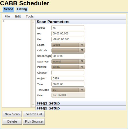
SourceThe name of the source. If the name of a calibrator in the ATCA calibrator database is entered into this field, the scheduler will automatically fill the
RA,Dec,EpochandCalCodefields. The information in this field will be used by the correlator as the name of the source in the output FITS files. If observing a mosaic, this field should be set to the name of the mosaic file describing the mosaic pointings, without the.mosextension.RA & DecThese fields define where on the sky you want the array to point, ie. the phase centre. You must specify
RAin hours, minutes and seconds separated by colons (:), and you must specifyDecin degrees, minutes and seconds separated by colons (:). TheRAandDecwill be in the system defined by theEpochfield, thus they can also be used to represent azimuth and elevation angles, and Galactic latitude and longitude.EpochThis defines the coordinate system used for the
RAandDecfields. Four epochs are recognised:J2000 (default)
B1950
Az/El (horizon coordinates)
Galactic
CalCodeA flag used to specify if a certain source is meant as a calibrator. It should either be “
C” for a calibrator, or blank for a non-calibrator. For baseline solutions, theCalCodeis set to “B”, a feature that should not be used by normal observers. When a calibrator is selected from the “Search Cal” screens, or matched from input to theSourcefield, this code will automatically be set to “C”. TheCalCodefield is reset to blank after a new scan is added to avoid inadvertantly calling a target source scan a calibrator scan.The assistance program makes use of the
CalCodefield to determine the level of on-line checking that is done. If a calibrator scan is indicated, the checks (for stable amplitude, small delays, closure phase, etc.) are more stringent. If a calibrator scan is not labelled with “CalCode=C” then these checks will not be performed. On the other hand, most target sources have structure and insufficient flux, so assistance would sound alarms continuously if a source like that was marked as a calibrator scan.ScanLengthThis indicates the length of time to spend on the current scan. It is specified in time format and should be specified as
HH:MM:SS, whereHH,MMandSSare the number of hours, minutes and seconds to spend on the source respectively. Unless theScanTypeis set toDwell, the scan time includes the time to drive to the source. The scan must be at least four integration cycles long.For many types of scan, this field is essentially meaningless, although it must always be set to four integration cycles or longer. For
Point,PaddleandClosefilescans, the scan will take as long as it needs to, and the setting of theScanLengthfield is unimportant.ScanTypeThis field specifies special scan characteristics:
Normal: the scan will go for the length of time specified byScanLength, inclusive of all slewing/setup time to get on source. For example, ifScanLengthis set to 10 minutes, then the scan will go for 10 minutes, even it takes 2 minutes to slew to source; in this case, only 8 minutes of data will be collected on-source.Dwell: the scan will go for the length of time specified byScanLength, in addition to any slewing/setup time incurred while moving to the source. For example, ifScanLengthis set to 10 minutes, and the telescope takes 2 minutes to slew to source, then this scan will go for 12 minutes, and 10 minutes of data will be collected on-source.Mosaic: this must be selected to indicate that this scan is a mosaic scan, and that theSourcefield should be interpreted as the name of a mosaic file.Point: indicates that this scan should be executed as a pointing pattern, which can be used to determine offsets for each antenna. This may be used for global pointing solutions as performed by local staff, or for reference pointing during observations.Paddle: indicates that the paddle should be inserted during 3mm observations; this scan type will have no effect during observations at other bands.Closefile: placing a scan with this scan type in a schedule causes the correlator to close the current file when it reaches this scan. No other scan parameters are interpreted when this scan type is specified. This is useful for keeping file sizes small, or for separating files based on the number of times the schedule has looped. The correlator will automatically start a new file when the next scan begins.OTFMos: this must be selected to indicate that this scan is an on-the-fly mosaic scan, and that theSourcefield should be interpreted as the name of a mosaic file.
PointingThis field specifies the pointing mode of the antenna during the scan. Options are:
Global: the default pointing mode. It uses the global, all-sky pointing model determined at each reconfiguration.Offset: uses the offsets from the latest pointing solution (which should be determined on a nearby calibrator) to improve the pointing locally (near the calibrator) and for a limited time (offsets are time variable). For experiments that track only a single source and a nearby calibrator, this is the safest pointing mode to use.Offpnt: instructs caobs to find the best pointing solution for this scan by looking through all pointing solutions from the previous two hours, and selecting the one closest in az/el position and frequency. If no suitable pointing solution is found, it reverts to the global pointing model, which may cause serious problems, especially at 3mm wavelengths. This mode should be preferred overOffsetpointing if many widely-separated sources are being observed together.Refpnt: determine new local pointing offsets by executing a pointing pattern on a calibrator. Using thisPointingmode causes the telescope to be put into global pointing mode before the new offsets are determined. This option only makes sense when combined with aScanTypeofPoint, and this should only be done while observing a calibrator.Setting
PointingtoRefpntwill make the scheduler automatically set theScanTypetoPoint.Update: determine new local pointing offsets by executing a pointing pattern on a calibrator. Using thisPointingmode causes the newly determined offsets to be added to the previously determined pointing solution. This option only makes sense when combined with aScanTypeofPoint, and this should only be done while observing a calibrator.Setting
PointingtoUpdatewill make the scheduler automatically set theScanTypetoPoint.
If you choose to have a
ScanTypeofPointand aPointingthat is notUpdate, the scheduler will popup a query box asking if you are sure this is what you want. For normal observations, you should always havePointing=UpdateforScanType=Pointso that the pointing offsets determined during the pointing scan will be used for all subsequentOffsetandOffpntscans. There may be other cases where the observer does not want the pointing to be automatically updated (such as during an array reconfiguration), which is why this option is not strictly forbidden.ObserverThis is an ASCII string up to 12 characters long that is used to identify who made the observations. It is not critical to any on-line system and is merely a label for reference.
ProjectThis is the project identification number (
nnn) allocated to observing projects, and should be specified here asCnnn. TheProjectfield value is used by cacor to name the extension of the output RPFITS files. It is important that it is set correctly as it is used for record keeping and by the ATNF Online Archive. The defaultC999code is used for system testing and test files; such files will not be considered as valuable when it comes to deleting data.The scheduler will complain if you enter a schedule file that doesn't look like
Cnnn,CXnnnorVnnna(the latter being a VLBI project code). You can choose to ignore the warning, and the scheduler will save the schedule, but it is strongly advised that you do not use a project code that does not fit the above pattern.TimeThe value of this field can only be set for source 1 in the schedule, and is used as the start time of the schedule. If
TimeCodeis set toLST, then this value is only used for calculation of slew times and elevations by the scheduler's listing tab, and will be ignored by caobs. IfTimeCodeis set toUTChowever, caobs will treat the schedule as an absolute time schedule, so each scan will only be executed between the time specified here (on the date specified in theDatefield) and the time plus the value inScanLength. This will usually only be useful when coordinating the activities of the ATCA with other telescopes (such as for VLBI).TimeCodeThe selection made here sets the type of time desired for the
Timefield above. It can be either local sidereal time (LST) or coordinated universal time (UTC). This field can only set for source 1 in the schedule. See the description of theTimefield for the consequences of setting this field to UTC.DateThe observing date can be set here to allow the scheduler to correctly determine the source positions and drive times. Of course, the date does not matter when setting LST, but is of vital importance when the
TimeCodeis set to UTC.This field is also used when the scheduler calculates the apparent frequency of a spectral line, which will be affected by the velocity of the Earth on the date specified here.
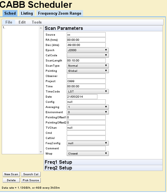
ConfigThe value of this field may (eventually) be used to configure the correlator. Currently, there are only a few easily-usable correlator configurations, and this field should be left blank, or given the default value of
null.AveragingThis parameter specifies the number of cycles to average together when writing the data out to an RPFITS file on disk. Averaging will restart on source and frequency changes. We do not recommend that this field is set to values larger than
1.EnvironmentSetting this field requests caobs to record the attenuator and sampler settings assocated with each different field value, and recall those settings whenever a scan is encountered with the same value. Each frequency setting (modulo 1 MHz) allows for up to 128 such values. Valid
Environmentvalues are from 0 to 127.PointingOffset1 & PointingOffset2Use these fields and the
OffpntPointingtype to make the telescope point away from the specified RA & Dec.PointingOffset1is the offset in seconds to move in RA, andPointingOffset2is the offset in arcseconds to move in Dec. Remember that the phase centre of the observation will always be at the position given in theRAandDecfields. Therefore if you wish to use these offset pointing fields to avoid a potential DC offset issue, you must put an offset position inRA,Decand then usePointingOffset1andPointingOffset2to shift the pointing centre to be on source again.TVChanWhen switching between different observing frequencies, the usable range of correlator channels will also change, due to RFI or bandpass shape. The correlator uses only a certain subset of channels – called the TV channels – to determine system temperatures, and if the TV channels are not kept constant for each individual frequency config then you may encounter amplitude problems later in the reduction process. The TV channels setting also affects what is displayed by vis. This parameter allows you to set the TV channels on a per scan basis, which makes frequency switching a far more automated process. This parameter should be either
nullto allow the current TV channel setting to be left as-is, or a set of four numbers, separated by commas, indicating (in order) the first and last TV channel for IF 1, and the first and last TV channel for IF 2.During normal frequency-switching observations, cacor will itself remember the TV channels on a per-frequency basis, and restore them as the frequencies change. If everything works as expected, this scheduler field is not required. This field is here in case you don't want to rely upon cacor's memory.
CmdThis field can be used to instruct caobs to issue one or more commands each time it starts this scan. Multiple commands may be specified, separated by semi-colons, although this field has an 80 character limit. Each command must be a recognised caobs command. For example, the tied-array configuration could be changed by specifying
corr catie ant 123456 123456; corr catie gain 0.2 0.2The first command listed in this field will be executed as soon as the scan is started, and each subsequent command will be executed as soon as the previous has been processed. To allow more flexibility in the timing of the commands listed in this field, there is a special command
WAIT n. This command (which cannot be used in manual caobs operation), waits fornintegrations after the start of the scan. After this condition has been met, the commands after theWAITcommand are executed. For example, to calibrate the phases after 5 cycles (to allow for data collection), specifywait 5; corr pcalThere are important caveats on the
WAITcommand. It does not guarantee on-source cycles will be waited: if the commandwait 5is specified, but it takes 5 or more cycles before the telescope gets on-source, the subsequent command will likely be executed before valid data is collected. To guard against this, consider putting a dummy scan before the scan with the command specification. The dummy scan should have a small (one or two cycles) amount of dwell time so that caobs will wait until the telescope is on-source before proceeding to the next scheduled scan.The
WAITcommand is not a progression command either. Take for example the following command:wait 5; corr dcal; wait 4; corr pcalThis command will fail to do what you might naively expect, because after thedcalcommand is issued, it will immediately issue thepcalcommand. This is because thewait 4command will immediately exit, as caobs has already waited for the fifth cycle to start, so it will no longer wait for the fourth cycle. Instead, this command should be:wait 5; corr dcal; wait 9; corr pcalCatVelThe
CatVelfield can be set manually, or via the scheduler's "Pick Source" function. This allows for rapid and reliable frequency calculation with the scheduler's velocity calculator, as the information in this field is automatically propagated into the calculator. This field should be set as three values, separated by spaces as follows:velocity velframe velconv
Here,
velocityis the velocity of the source in km/s (recession is positive),velframeis the frame in which the velocity is measured (one ofLSRorBary), andvelconvis the velocity convention (one ofRadio,OpticalorZ).This field must be set if you want to use the scheduler's zoom range checker.
FreqConfigThe
FreqConfigfield is used to create a number of frequency and zoom settings that can be shared between scans. Setting the continuum frequencies and specifying up to 16 zooms in each IF can be tedious and error prone if it has to be repeated for many scans. TheFreqConfigfield lets you select one or more scans asMasterscans and then assign other scans to beSlavescans. EachSlavescan inherits the exact frequency and zoom settings of the correspondingMasterscan. Using this you can ensure source and calibrator are observed with the same settings, even after recalculating velocities and frequencies for a different date. The default setting ofnullleaves the settings independent of other scans.CommentThis field can be used to leave comments for yourself in the schedule. It is it not used on-line, nor is this entry available outside the scheduler.
WrapThe ATCA can be in one of two “wraps”, and the azimuth ranges observable in each wrap are different, although they overlap. This field can be used if you want to control which wrap to use for your observations. It can take one of three values:
Closest,SouthorNorth. See Section 2.3.10 for a description of the wraps.
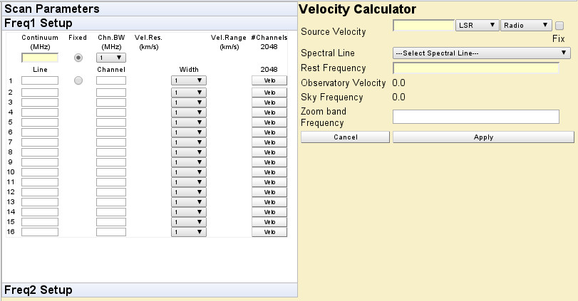
Continuum (MHz)Enter the central frequency (in MHz) of the 2048 MHz continuum IF here. There is one of these fields in each of the
Freq1andFreq2tabs, one for each available CABB continuum IF. If after entering a frequency in this box, the box text turns red on a yellow background, it means the frequency is invalid when considered with the frequency specified in the other IF. Putting the mouse over the frequency box will give you some information on how you might rectify this situation.Chn. BW (MHz)Select how wide (in MHz) each continuum channel will be for each IF. The channel width will also set the minimum bandwidth of each zoom band derived from this IF. There is one of these fields in each of the
Freq1andFreq2tabs, one for each available CABB continuum IF.LineEnter a frequency (in MHz) that will appear within the zoom band. The scheduler will then calculate the continuum (or offset continuum) channel that would have this specified frequency closest to its centre. This frequency must be within 1024 MHz of the frequency specified in the
Continuum (MHz)field. A maximum of 16 such bands can be specified in the scheduler for each IF when using a channel bandwidth of 1 MHz or 64 MHz.ChannelEnter the wideband channel number to use for the zoom band. This will then restrict the frequencies available in the zoom band.
WidthThis is the number of continuum channels to use for this zoom band. Note that a maximum of 16 continuum channels can be used in each IF. Some of the
Widthboxes will be disabled if more than 1 continuum channel is assigned to any particular zoom band.FixedUse this to select whether to keep the continuum frequency fixed or keep the frequency of the first zoom fixed when you change the
Channel,Widthor velocity.VeloThis button brings up the velocity calculator that lets you specify the source velocity and rest frequency to calculate the sky frequency of the spectral line. The sky frequency is rounded to the nearest possible frequency setting of the telescope and entered in the schedule when you press the
Applybutton.FixThis tick box appears on the velocity calculator. When ticked, the same velocity setting will be used for all zooms on both frequencies. Use this to avoid having to enter the same information many times when the source has many spectral lines with more or less the same velocity.
The following buttons are available on the main scheduler page.
New ScanThis button duplicates the currently selected scan and inserts it as the next scan in the schedule, and moving all subsequent scans down by one. The duplicated scan will however have its
CalCodereset.DeleteThis button deletes the currently selected scan, and moves all subsequent scans up by one.
Search CalThis button initiates a search through the ATCA calibrator database for calibrators within 20 degrees of the position of the currently selected scan, with a flux density greater than 125 mJy in the frequency band you have specified. The results of this search are displayed to the right of the scan parameters, and are sorted by distance to the selected scan's position. Each calibrator returned by this search can be viewed in detail by clicking the button next to the calibrator's name, and it can be inserted at the currently selected position in the schedule by clicking on the button twice in succession.
Please note that after clicking the source name button, it can take up to a minute before the detailed flux density history of the source is shown, although it is usually significantly faster than that.
Pick SourceClick this button to load in a file from your own computer containing sources that will be used in the schedule. After clicking on this button, a new frame will appear next to this button allowing the selection of a locally-hosted file with the format:
source_name hh:mm:ss.s dd:mm:ss.s epoch [vel velframe velconv]
...
This file may have any number of sources, with one source listed per line, along with its RA (in hh:mm:ss.s format), Dec (in dd:mm:ss.s format), and coordinate Epoch separated by spaces. The Epoch must be one of those supported by the scheduler; currently these are
J2000,B1950,AzElandGalactic. The velocity of each source can optionally be specified in km/s, along with the velocity frame (one ofLSRorBary), and the velocity convention (one ofRadio,OpticalorZ).Click the
Submitbutton to load in this file. After the file is loaded, a Source Selection frame will appear to the right of the Scan Parameters, and each source will be listed, with buttons for each source in the file. Clicking on the button labelled with the source name will insert that source into the schedule at the currently selected scan number, and move all subsequent scans down by one. Clicking theAddAllbutton will add all the scans to the schedule, in order, at the currently selected scan number, and will move all subsequent scans down by the number of sources in the Source Selection frame. The sources that are added will have the same scan parameters and frequencies that the currently selected source has.SchedSelecting this tab will show the schedule editing functions.
ListingSelecting this tab will generate a time-ordered summary of scans from the current schedule. It is most useful for checking the validity and correctness of the schedule. It will look something like Figure F.4.
For each scan in the schedule, the listing view gives the following information.
#The scan number in the schedule.
SourceThe name of the source.
CalThis column will be blank if the calibrator code is not set, or
CorBif the appropriate calibrator code is set.RAThe right ascension of the scan.
DecThe declination of the scan.
EpochThe epoch of the position.
TimeThe time at the start of the scan. If the
TimeCodeof the schedule is LST then this is shown as LST; likewise with UTCTimeCodes.The time at the start of the first scan is always the same as is specified in the
Timefield for that scan. For subsequent scans the time here includes the time spent on the previous scan and the time required to slew from the previous position to this position.Note that it will not necessarily be accurate when the previous scan is a pointing, paddle or mosaic scan, where the
ScanLengthis not necessarily representative of the actual time spent on the scan.ScanLengthThe length of the scan, in hours, minutes and seconds listed as
hh:mm:ss. This is only what is listed in the scheduler, and does not consider the actual amount of time that will be spent on the scan if it is a mosaic, pointing or paddle scan.AzThe azimuth of the source at the time listed in the
Timecolumn, in degrees, minutes and seconds.ElThe elevation of the source at the time listed in the
Timecolumn, in degrees, minutes and seconds.DriveThe time required to slew to the source from the previous scan position. For the first scan, the drive time is the time required to slew from the stow position.
If the elevation of the source is below 12° then the drive time is shown as
00:00:00because of course the telescope cannot perform the scan.WrapThis column will only be present if the scheduler is in the advanced view mode. The wrap that is specified in the scheduler
Wrapis displayed here; it does not compute what the wrap will actually be during the observations.ScanTypeThe type of scan (eg. dwell, point, paddle etc.).
PointingThe pointing solution to use for the scan.
Freq-1The centre frequency of the CABB continuum IF1, in MHz.
Freq-2The centre frequency of the CABB continuum IF2, in MHz.
ChnBW-1The width of each continuum channel in IF1, in MHz. This column will only be present if the scheduler is in the advanced view mode.
ChnBW-2The width of each continuum channel in IF2, in MHz. This column will only be present if the scheduler is in the advanced view mode.
FreqCfgThis column will show whether the scan has been assigned as a master frequency scan, or if it is slave to another scan. If the column is blank, or
nullthen it is neither a master or a slave.This column will only be present if the scheduler is in the advanced view mode.
CatVelThe velocity as specified in the scheduler's
CatVelfield. This column will only be present if the scheduler is in the advanced view mode.AverThe number of cycles that will be averaged together for this scan. This column will only be present if the scheduler is in the advanced view mode.
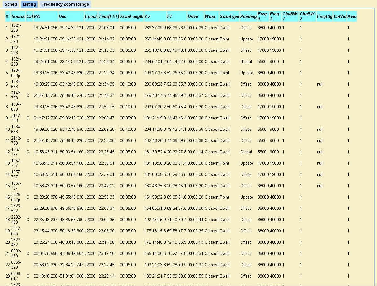
The scheduler has three drop-down menus, which are described below.
FileThe
Filemenu has the following items.OpenOpens a pre-existing schedule from the server.
SaveSaves the schedule with the name that it already has. If the schedule does not currently have a name, this action will not work. This action saves the schedule to the server, ready for loading in caobs.
SaveAsAllows the schedule to be saved with a different name than it currently has. If the schedule does not currently have a name, this action is the only way to save it to the server.
OpenLocalLoad a schedule that you have saved on your local computer (instead of from the common schedule area that caobs can access). When this action is selected, a file selection area will appear at the bottom of the scheduler screen asking you to
Select schedule file. Use theBrowsebutton to find the schedule you want to load and then click theSubmitbutton, or press theCancelbutton to cancel this action.SaveLocalSaves the schedule to your local computer (instead of to the common schedule area that caobs can access). Use this option if you're not ready to, or not able to (due to ATNF access restrictions) save to the remote server. You will be prompted to save a file called
cabb.schon your local disk.CloseCloses the current schedule and resets the interface back to an empty schedule with 1 generic scan and no schedule name.
EditThe
Editmenu has the following items.CutRemoves the currently selected scans from their position in the schedule, but keeps it in memory so that they can be inserted elsewhere.
CopyCopies the currently selected scans into memory so that they can be inserted elsewhere.
PasteCopies the scan information held in memory from a prior
CutorCopyaction back into the schedule, as scans after the currently selected scan. This moves all subsequent scans down by the number of scans that are pasted in. It is not possible toPastea scan into position 1 in the schedule.
ToolsThe
Toolsmenu has the following items.Advanced ViewThis menu item will only be present if the scheduler is currently in “Simple View”. Selecting it will make the scheduler display more fields than are strictly required to make a simple schedule.
Simple ViewThis menu item will only be present if the scheduler is currently in “Advanced View”. Selecting it will make the scheduler display on the fields that are strictly required to make a simple schedule. However, all of the advanced fields will retain their settings irrespective of the scheduler view mode.
Global changeAllows a change in one scan to be duplicated in all other scans. The scan/scans to change should be selected first, followed by the
Global changemenu item. While the global change mode is activated, it is not possible to change the set of selected scans. Make as many changes to the scan as is necessary, in any of theScan Parameters,Freq1andFreq2tabs, and then select either theGlobal Applybutton to confirm the changes and duplicate them in all the other scans in the schedule, or theGlobal Cancelbutton to keep the changes but do not duplicate them.The button
Global Apply Selectedis used to effect the changes only to the scans that were selected before entering global change mode.The button
Global Apply Matchingis used to duplicate the changes only to other scans that initially matched the scan being changed. An example of this is for a schedule that has multiple frequencies in a single IF. Consider a schedule that has scans with IF1 frequencies of 5500, 5700 and 8600 MHz. If a scan with an IF1 frequency of 8600 MHz is changed to 8700 MHz, and theGlobal Applybutton is used, then all scans in the schedule will be changed to have an IF1 frequency of 8700 MHz. However, if theGlobal Apply Matchingbutton is used, then only scans that have an IF1 frequency of 8600 MHz, like the selected scan, will be changed.It is also important to note that if nothing changes, then using the
Global Applybutton will not do anything. For example, if a scan is changed individually fromProject=C123toProject=C124, and this change needs to propagate to all scans, then simply deleting the entry in this scan and replacing it with the same thing while inGlobal changemode will not work, as it will still appear as though the entry has not changed. Instead, move to another scan where theProjectcode has not changed before enteringGlobal changemode.Another important caveat is that even though more than one scan can be selected before entering global change mode, only the parameters of the first selected scan will be displayed in the scheduler fields.
Recalc freq/veloGoes through the schedule and recomputes all frequency and velocity information present. This is useful to execute when you change the
Datefield, to ensure that all the zoom mode information is correct.Load local catalogUse this menu item to load a catalogue of sources from a local machine into the scheduler, which can then be inserted into the schedule with the
Pick Sourcebutton.If the
Pick Sourcebutton is used before a local catalog is loaded, then a frame allowing a catalog is shown. However, after this catalog is loaded, subsequent selections of thePick Sourcebutton will display only theSource Selectionframe. To show the catalog loading frame again, so that a different catalog can be loaded, use theLoad local catalogmenu item.Load remote catalogUse this menu item to load a catalogue of sources from the remote database into the scheduler, which can then be inserted into the schedule with the
Pick Sourcebutton. These remote catalogues include the VLA and AT calibrator catalogues, among others.
Use new cal databaseIf this menu item is present, then the
Search Calbutton will be querying the old calibrator database for calibrator positions and fluxes. Selecting this menu item will make the web scheduler query the new calibrator database whenever theSearch Calbutton is pressed.Use old cal databaseIf this menu item is present, then the
Search Calbutton will be querying the new calibrator database for calibrator positions and fluxes. Selecting this menu item will make the web scheduler query the old calibrator database whenever theSearch Calbutton is pressed.
For accurate work, Cartesian (XYZ) coordinates are much to be preferred, since the use of latitude, longitude and height entails a number of possible uncertainties and ambiguities. In particular, there are two families of commonly-used geodetic coordinate systems (lat/long/height) that can differ by as much as 200m. (The fact that the ATCA site survey in 1984 fell into just this trap emphasises the point.)
The choice of the correct type of geodetic coordinate depends on the application. In most cases, the geocentric WGS84 given below will probably be appropriate (eg in the calculation of LST). The non-geocentric system AGD84/AHD currently used by Australian cartographers and surveyors is unlikely to be relevant for astronomy, but is included for completeness and to allow comparison with existing physical surveys.
| Ref | X(m) | e(X) | Y(m) | e(Y) | Z(m) | e(Z) |
|---|---|---|---|---|---|---|
| W196 | -4750915.837 | ∼2 | 2792906.182 | ∼2 | -3200483.747 | ∼2 |
| W196_vlbi | -4750924.9 | ∼2 | 2792911.5 | ∼2 | -3200489.9 | ∼2 |
| MOPRA | -4682768.1 | ∼1 | 2802618.8 | ∼1 | -3291759.2 | ∼2 |
| PARKES | -4554231.533 | .031 | 2816759.109 | .018 | -3454036.323 | .025 |
Notes: The coordinates are in a conventional geocentric right-handed Cartesian system, with the Z axis parallel to the mean rotation axis (North) and the X-axis aligned towards the intersection of the Greenwich meridian and the equator.
W196 refers to the centroid of the four pier-tops of station W196 of the ATCA. The listed position is that currently in use by CAOBS in the STATION.COORDINATES file. The position is derived from a physical survey (pre-GPS: see ATNF documents AT/15.6.1/001-003, AT/15.6.2/012) and is uncertain at the ∼2m level although the relative positions of the CA stations are accurate at the ∼mm level. The reference frame of the survey is unstated, but is probably AGD66. However, for consistency with existing coordinates in use at the ATCA it is assumed to be AGD84 (∼2m differences against AGD66). The geoidal height used in the survey (N[ANS]=11.4m) has also been retained for consistency (though more accurate estimates are since available).
The antenna coordinates used by CAOBS for array pointing prior to October 1991 were all approximately 200m in error (mostly a uniform translation) owing to a misconception of references systems in the surveyors' report. The coordinates currently in use are consistent with the position given here for W196.
Station W196 is the logical choice to define a single position for the entire array. It is exactly midway between the two outer stations (W0 and W392) and is the only station for which the four support piers lie in the true local horizontal plane to make the antenna azimuth axis strictly vertical. It should therefore be used to define local sidereal time (LST) for the whole array so that all antenna azimuth and elevation angles are consistent. (The azimuth axes of antennas on the other stations are all parallel to that of station W196 and are therefore progressively tilted from the vertical.)
W196_vlbi refers to a point 10 metres above the centroid of the pier tops, approximating the position of the intersection of the elevation and azimuth axes (relevant for VLBI). A more accurate estimate of the geoidal height has also been used (N[ANS]=13.5m or N[WGS84]=29.7m, based on OSU86E). This position will be improved by further VLBI observations (once an H-maser is available).
The MOPRA and Parkes positions both derive from VLBI measurements and hence refer in both instances to the point of axial intersection. The Parkes position was obtained from S/X Mark-III VLBI data in January 1992 (Parkes-Hobart-DSS45) and is nominally on the ITRF frame. The Mopra position was derived from 4.8 GHz Mark-II data from May 1993.
| Ref | Longitude | Latitude | Spheroidal |
|---|---|---|---|
| (degs/dms) | (degs/dms) | Height (WGS84) | |
| W196 | 149.5501388 | -30.3128846 | 236.87m |
| 149 33 00.500 | -30 18 46.385 | ||
| MOPRA | 149.0996405 | -31.2678132 | 866.44m |
| 149 05 58.706 | -31 16 04.127 | ||
| PARKES | 148.2635101 | -32.9984064 | 414.80m |
| 148 15 48.636 | -32 59 54.263 |
Notes: these figures are derived from the preceding Cartesian coordinates using the WGS84 figure for the Earth. This is close to the frame often used by GPS but note that some GPS receivers display position data in local coordinate systems (eg AGD84/ANS).
| Ref | Longitude | Latitude | AHD height |
|---|---|---|---|
| (degs/dms) | (degs/dms) | (above sea level) | |
| W196 | 149.5489798 | -30.3144576 | 209.30m |
| 149 32 56.327 | -30 18 52.048 | ||
| MOPRA | 149.0984643 | -31.2693808 | 837.94m |
| 149 05 54.472 | -31 16 09.771 | ||
| PARKES | 148.2623007 | -32.9999629 | 391.52m |
| 148 15 44.283 | -32 59 59.866 |
Notes: The figures are derived from geocentric Cartesian coordinates using the Higgins (1987) seven-parameter transformation of WGS84 to AGD84. The latter is a coordinate system specific to Australia, using a non-geocentric spheroidal fit to the local geoid (the ANS, or Australian National Spheroid). The AHD height is height above mean sea-level or (equivalently) height above the geoid. For Narrabri, the AHD is that quoted in the surveyors' report (AT/15.6.1/003, AT/15.6.2/012). For Parkes and Mopra, values of N[WGS84] (height of the geoid above the WGS84 spheroid) are were interpolated on AUSGEOID93 (from OSU91).
Latitudes and longitudes read from Australian topographic maps are invariably in the above system or a precursor (eg AGD66). Some GPS receivers also allow positional data to be displayed in this system.
The names of Station Posts on the East-West track are generated from their distance, in multiples of 15.306 metres, from the eastern most station post on the Compact Array (W0). Similarly, the names of station posts on the North Spur are generated from their increment from the southernmost station post on the north spur (W106).
| Station | d (m) | Old name |
|---|---|---|
| W0 | 0.000 | (Station 1) |
| W2 | 30.612 | (Station 2) |
| W4 | 61.224 | (Station 3) |
| W6 | 91.837 | (Station 4) |
| W8 | 122.449 | (Station 5) |
| W10 | 153.061 | (Station 6) |
| W12 | 183.673 | (Station 7) |
| W14 | 214.286 | (Station 8) |
| W16 | 244.898 | (Station 9) |
| W32 | 489.796 | (Station 10) |
| W45 | 688.776 | (Station 11) |
| W64 | 979.592 | (Station 12) |
| W84 | 1285.714 | (Station 13) |
| W98 | 1500.000 | (Station 14) |
| W100 | 1530.612 | (Station 15) |
| W102 | 1561.224 | (Station 16) |
| W104 | 1591.837 | |
| W106 | 1622.449 | |
| W109 | 1668.367 | (Station 17) |
| W110 | 1683.673 | (Station 18) |
| W111 | 1698.980 | (Station 19) |
| W112 | 1714.286 | (Station 20) |
| W113 | 1729.592 | (Station 21) |
| W124 | 1897.959 | |
| W125 | 1913.265 | |
| W128 | 1959.184 | (Station 22) |
| W129 | 1974.490 | (Station 23) |
| W140 | 2142.857 | (Station 24) |
| W147 | 2250.000 | (Station 25) |
| W148 | 2265.306 | (Station 26) |
| W163 | 2494.898 | (Station 27) |
| W168 | 2571.429 | (Station 28) |
| W172 | 2632.653 | (Station 29) |
| W173 | 2647.959 | (Station 30) |
| W182 | 2785.714 | (Station 31) |
| W189 | 2892.857 | (Station 32) |
| W190 | 2908.163 | (Station 33) |
| W195 | 2984.694 | (Station 34) |
| W196 | 3000.000 | (Station 35) |
| W392 | 6000.000 | (Station 37) |
| N2 | 30.612 | |
| N5 | 76.531 | |
| N7 | 107.143 | |
| N11 | 168.367 | |
| N14 | 214.286 |
Notes:
Antennas 1 to 5 are confined to stations W0 to W196 and N spur stations. Antenna 6 is permanently stationed on station W392. Antennas must be separated by ≥30 m.
d is the distance in metres from W0 at the eastern end of the array, or, for N stations, the distance from the EW track.
Old names were used before 2002.
Each of the ATCA's possible array configurations are listed below. For each array, the station locations are listed for each antenna, and whenever an antenna can be located on multiple stations in that configuration, all the variants that have been used are listed. For the most used variant of each configuration, the baseline lengths are shown, in metres.
Configurations within each group of 4 (ie. 6A, 6B, 6C, 6D), or in one of the complementary array groups (designated as a, b, c, d and e) form complementary sets for multi-day observations. Note: This is for single-frequency observations. For a more sophisticated approach, see the section on bandwidth and multi-frequency synthesis.
CA06 sits permanently on station W392. Baselines to this antenna are shown for all configurations, but form part of the design only for the 6 km configurations (6A, 6B, 6C and 6D).
- Array: 6A
This array is part of the a and b complementary array groups.
Variant CA01 CA02 CA03 CA04 CA05 CA06 6A W4 W45 W102 W173 W196 W392 Baseline lengths are in metres.
6A CA02 CA03 CA04 CA05 CA06 CA01 627.6 1500.0 2586.7 2923.5 5938.8 CA02 872.40 1959.2 2295.9 5311.2 CA03 1086.7 1423.5 4438.8 CA04 336.7 3352.0 CA05 3015.3 - Array: 6B
Variant CA01 CA02 CA03 CA04 CA05 CA06 6B W2 W64 W147 W182 W196 W392 Baseline lengths are in metres.
6B CA02 CA03 CA04 CA05 CA06 CA01 949.0 2219.4 2755.1 2969.4 5969.4 CA02 1270.4 1860.1 2020.4 5020.4 CA03 537.7 750.0 3750.0 CA04 214.3 3214.3 CA05 3000.0 - Array: 6C
This array is part of the a and b complementary array groups.
Variant CA01 CA02 CA03 CA04 CA05 CA06 6C W0 W10 W113 W140 W182 W392 Baseline lengths are in metres.
6C CA02 CA03 CA04 CA05 CA06 CA01 153.1 1729.6 2142.9 2785.7 6000.0 CA02 1576.5 1989.8 2632.7 5846.9 CA03 413.3 1056.1 4270.4 CA04 642.9 3857.1 CA05 3214.3 - Array: 6D
Variant CA01 CA02 CA03 CA04 CA05 CA06 6D W8 W32 W84 W168 W173 W392 Baseline lengths are in metres.
6D CA02 CA03 CA04 CA05 CA06 CA01 367.3 1163.3 2449.0 2525.5 5877.5 CA02 795.9 2081.6 2158.2 5510.2 CA03 1285.7 1362.2 4714.3 CA04 76.5 3428.6 CA05 3352.0 - Array: 1.5A
Variant CA01 CA02 CA03 CA04 CA05 CA06 1.5A W100 W110 W147 W168 W196 W392 Baseline lengths are in metres.
1.5A CA02 CA03 CA04 CA05 CA06 CA01 153.1 719.4 1040.8 1469.4 4469.4 CA02 566.3 887.8 1316.3 4316.3 CA03 321.4 750.0 3750.0 CA04 428.6 3428.6 CA05 3000.0 - Array: 1.5B
This array is part of the a and b complementary array groups.
Variant CA01 CA02 CA03 CA04 CA05 CA06 1.5B W111 W113 W163 W182 W195 W392 Baseline lengths are in metres.
1.5B CA02 CA03 CA04 CA05 CA06 CA01 30.6 795.9 1086.7 1285.7 4301.0 CA02 765.3 1056.1 1255.1 4270.4 CA03 290.8 489.8 3505.1 CA04 199.0 3214.3 CA05 3015.3 - Array: 1.5C
This array is part of the a and c complementary array groups.
Variant CA01 CA02 CA03 CA04 CA05 CA06 1.5C W98 W128 W173 W190 W195 W392 Baseline lengths are in metres.
1.5C CA02 CA03 CA04 CA05 CA06 CA01 459.2 1148.0 1408.2 1484.7 4500.0 CA02 688.8 949.0 1025.5 4040.8 CA03 260.2 336.7 3352.0 CA04 76.5 3091.8 CA05 3015.3 - Array: 1.5D
This array is part of the b and c complementary array groups.
Variant CA01 CA02 CA03 CA04 CA05 CA06 1.5D W102 W109 W140 W182 W196 W392 Baseline lengths are in metres.
1.5D CA02 CA03 CA04 CA05 CA06 CA01 107.1 581.6 1224.5 1438.8 4438.8 CA02 474.5 1117.3 1331.6 4331.6 CA03 642.9 857.1 3857.1 CA04 214.3 3214.3 CA05 3000.0 - Array: 750A
This array is part of the c complementary array group.
Variant CA01 CA02 CA03 CA04 CA05 CA06 750A W147 W163 W172 W190 W195 W392 Baseline lengths are in metres.
1.5A CA02 CA03 CA04 CA05 CA06 CA01 244.9 382.7 658.2 734.7 3750.0 CA02 137.8 413.3 489.8 3505.1 CA03 275.5 352.0 3367.3 CA04 76.5 3091.8 CA05 3015.3 - Array: 750B
Variant CA01 CA02 CA03 CA04 CA05 CA06 750B W98 W109 W113 W140 W148 W392 Baseline lengths are in metres.
750B CA02 CA03 CA04 CA05 CA06 CA01 168.4 229.6 642.9 765.3 4500.0 CA02 61.2 474.5 596.9 4331.6 CA03 413.3 535.7 4270.4 CA04 122.4 3857.1 CA05 3734.7 - Array: 750C
Variant CA01 CA02 CA03 CA04 CA05 CA06 750C W64 W84 W100 W110 W113 W392 Baseline lengths are in metres.
750C CA02 CA03 CA04 CA05 CA06 CA01 306.1 551.0 704.1 750.0 5020.4 CA02 244.9 398.0 443.9 4714.3 CA03 153.1 199.0 4469.4 CA04 45.9 4316.3 CA05 4270.4 - Array: 750D
This array is part of the c complementary array group.
Variant CA01 CA02 CA03 CA04 CA05 CA06 750D W100 W102 W128 W140 W147 W392 Baseline lengths are in metres.
750D CA02 CA03 CA04 CA05 CA06 CA01 30.6 428.6 612.2 719.4 4469.4 CA02 398.0 581.6 688.8 4438.8 CA03 183.7 290.8 4040.8 CA04 107.1 3857.1 CA05 3750.0 - Array: EW367
This array is part of the d complementary array group.
Variant CA01 CA02 CA03 CA04 CA05 CA06 EW367 W104 W110 W113 W124 W128 W392 EW367B W124 W104 W110 W113 W128 W392 Baseline lengths are in metres.
EW367 CA02 CA03 CA04 CA05 CA06 CA01 91.8 137.8 306.1 367.3 4408.2 CA02 45.9 214.3 275.5 4316.3 CA03 168.4 229.6 4270.4 CA04 61.2 4102.0 CA05 4040.8 - Array: EW352
This array is part of the d complementary array group.
Variant CA01 CA02 CA03 CA04 CA05 CA06 EW352 W102 W104 W109 W112 W125 W392 EW352B W112 W102 W104 W109 W125 W392 Baseline lengths are in metres.
EW352 CA02 CA03 CA04 CA05 CA06 CA01 30.6 107.1 153.1 352.0 4438.8 CA02 76.5 122.4 321.4 4408.2 CA03 45.9 244.9 4331.6 CA04 199.0 4285.7 CA05 4086.7 - Array: EW214
Variant CA01 CA02 CA03 CA04 CA05 CA06 EW214 W98 W102 W104 W109 W112 W392 EW214B W109 W98 W102 W104 W112 W392 Baseline lengths are in metres.
EW214 CA02 CA03 CA04 CA05 CA06 CA01 61.2 91.8 168.3 214.2 4498.2 CA02 30.6 107.1 153.0 4437.0 CA03 76.5 122.4 4406.4 CA04 45.9 4329.9 CA05 4284.0 - Array: NS214
Variant CA01 CA02 CA03 CA04 CA05 CA06 NS214 W106 N2 N7 N11 N14 W392 Baseline lengths are in metres.
NS214 CA02 CA03 CA04 CA05 CA06 CA01 30.6 107.1 168.3 214.2 4377.5 CA02 76.5 137.7 183.6 4377.7 CA03 61.2 107.1 4378.9 CA04 45.9 4380.8 CA05 4382.8 - Array: H214
This array is part of the e complementary array group.
Variant CA01 CA02 CA03 CA04 CA05 CA06 H214 W98 W104 W113 N5 N14 W392 H214B W98 W104 N14 N5 W113 W392 H214C W98 N5 N14 W104 W113 W392 H214D W98 N14 N5 W104 W113 W392 Baseline lengths are in metres.
H214D CA02 CA03 CA04 CA05 CA06 CA01 246.8 144.4 91.8 229.6 4500.0 CA02 137.8 216.5 239.6 4382.8 CA03 82.4 131.7 4378.2 CA04 137.8 4408.2 CA05 4270.4 - Array: H168
This array is part of the e complementary array group.
Variant CA01 CA02 CA03 CA04 CA05 CA06 H168 W100 W104 W111 N7 N11 W392 H168B W100 W104 N11 N7 W111 W392 H168C W100 N7 N11 W104 W111 W392 H168D W100 N11 N7 W104 W111 W392 Baseline lengths are in metres.
H168D CA02 CA03 CA04 CA05 CA06 CA01 191.8 141.1 61.2 168.4 4469.4 CA02 61.2 171.1 184.9 4380.8 CA03 111.4 131.7 4378.9 CA04 107.1 4408.2 CA05 4301.0 - Array: H75
This array is part of the e complementary array group.
Variant CA01 CA02 CA03 CA04 CA05 CA06 H75 W104 W106 W109 N2 N5 W392 H75B W104 N5 N2 W106 W109 W392 H75C W104 N2 N5 W106 W109 W392 Baseline lengths are in metres.
H75C CA02 CA03 CA04 CA05 CA06 CA01 43.3 82.4 30.6 76.5 4408.2 CA02 45.9 30.6 55.2 4377.7 CA03 76.5 89.2 4378.2 CA04 45.9 4377.5 CA05 4331.6 - Array: 122C
Variant CA01 CA02 CA03 CA04 CA05 CA06 122C W98 W100 W102 W104 W106 W392 Baseline lengths are in metres.
122C CA02 CA03 CA04 CA05 CA06 CA01 30.6 61.2 91.8 122.4 4498.2 CA02 30.6 61.2 91.8 4467.6 CA03 30.6 61.2 4437.0 CA04 30.6 4406.4 CA05 4375.8 - Array: 375
This is an obsolete array.
Variant CA01 CA02 CA03 CA04 CA05 CA06 375 W2 W10 W14 W16 W32 W392 Baseline lengths are in metres.
375 CA02 CA03 CA04 CA05 CA06 CA01 122.4 183.6 214.2 459.0 5967.0 CA02 61.2 91.8 336.6 5844.6 CA03 30.6 275.4 5783.4 CA04 244.8 5752.8 CA05 5508.0 - Array: 210
This is an obsolete array.
Variant CA01 CA02 CA03 CA04 CA05 CA06 210 W98 W100 W102 W109 W112 W392 Baseline lengths are in metres.
210 CA02 CA03 CA04 CA05 CA06 CA01 30.6 61.2 168.3 214.2 4498.2 CA02 30.6 137.7 183.6 4467.6 CA03 107.1 153.0 4437.0 CA04 45.9 4329.9 CA05 4284.0 - Array: 122A
This is an obsolete array. Prior to July 1996, this configuration was known as 122.
Variant CA01 CA02 CA03 CA04 CA05 CA06 122A W0 W2 W4 W6 W8 W392 Baseline lengths are in metres.
122A CA02 CA03 CA04 CA05 CA06 CA01 30.6 61.2 91.8 122.4 5997.6 CA02 30.6 61.2 91.8 5967.0 CA03 30.6 61.2 5936.4 CA04 30.6 5905.8 CA05 5875.2 - Array: 122B
This is an obsolete array. Prior to July 1996, this configuration was known as 120.
Variant CA01 CA02 CA03 CA04 CA05 CA06 122B W8 W10 W12 W14 W16 W392 Baseline lengths are in metres.
122B CA02 CA03 CA04 CA05 CA06 CA01 30.6 61.2 91.8 122.4 5875.2 CA02 30.6 61.2 91.8 5845.0 CA03 30.6 61.2 5814.8 CA04 30.6 5784.6 CA05 5754.4
The diagrams in this section can allow you to quickly determine how long you can observe a source with a particular array before you have problems with shadowing.
These diagrams are to read as follows.
The grey area on each plot is where the source is above the 12° elevation limit and there is no shadowing on any antenna.
For any source at a particular declination, you can determine the hour angle at which the source sets, or an antenna becomes shadowed, by reading off the hour angle at the edge of the grey area. The hour angle for the elevation limit or shadowing is symmetrical around zero.
Each of the hybrid arrays has its own shadowing diagram, but you can use the first diagram for any east-west array with baselines shorter than 61.2 m.
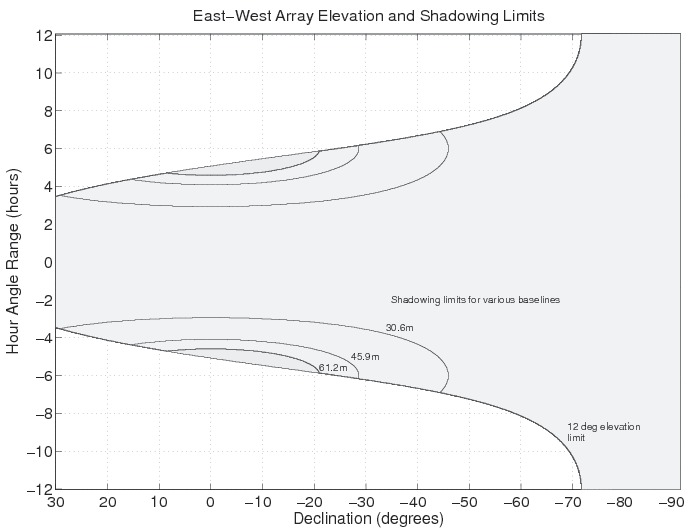
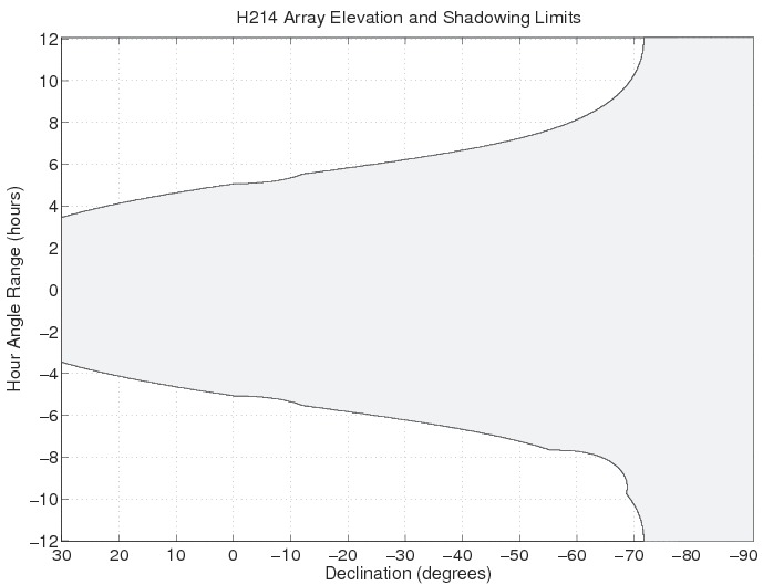
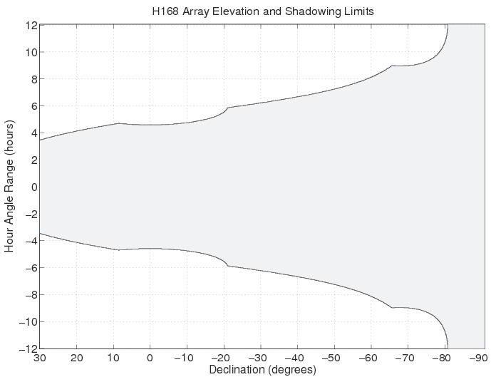
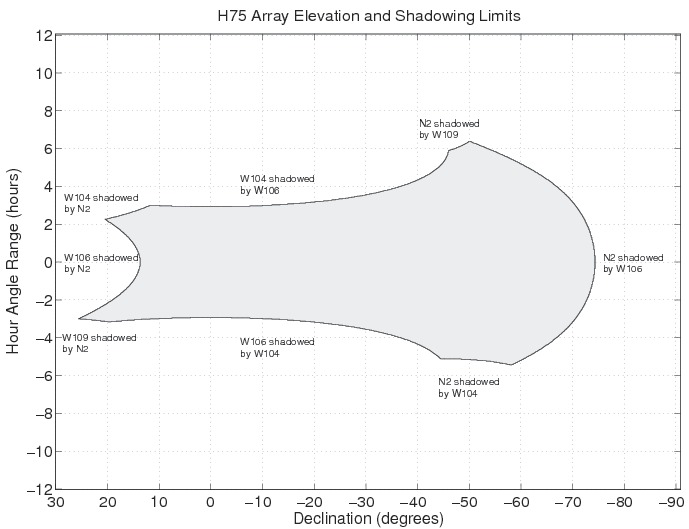
A
- amplifier
- HEMT, Online Calibration
- low noise, Online Calibration
- MMIC, Online Calibration
- antenna
- focus, Design and Operation of the ATCA
- optics, Design and Operation of the ATCA
- reference, cacor Commands
- station locations, Station Locations
- surface, Design and Operation of the ATCA
- temperature, Sensitivity and System Temperature
- wrap limits, What are the antenna “wraps”?
- array
- configurations, Array configurations
- tied, Tied Array Mode
- ASKAP, The Australia Telescope National Facility
- ATCA, The Australia Telescope Compact Array
- baselines, Array configurations, Sensitivity and System Temperature
- calibration, Online Calibration
- configurations, Array configurations, Sensitivity and System Temperature, Array Configurations and Baselines
- coordinates, Observatory Coordinates
- declination coverage, How long is my source up per day?
- field of view, Sensitivity and System Temperature
- forum, Read this First
- frequencies, Sensitivity and System Temperature
- longitude & latitude, Overview of the ATCA
- overview, Overview of the ATCA
- station locations, Station Locations
- subreflector, Focus
- ATNF, The Australia Telescope National Facility
- headquarters, The Australia Telescope National Facility
- attenuators
- levels
B
- band, Design and Operation of the ATCA, Sensitivity and System Temperature
- letter codes, Design and Operation of the ATCA
- splitter, Online Calibration
- bandwidth, Sensitivity and System Temperature
- baselines (see ATCA)
C
- CABB
- bad channels, How do I best map regions of spectral line emission?
- birdies, How do I best map regions of spectral line emission?
- blocks, CABB Correlator
- boards, CABB Correlator
- delay units, CABB Correlator
- digitisers, Online Calibration, CABB Correlator, Artefacts
- installation, Bandwidths and correlator
- reprogramming
- 1MHz no zooms, Changing to 1MHz, No Zooms
- 1MHz zooms, Changing to 1MHz Zooms
- 64MHz zooms, Changing to 64MHz Zooms
- generic, Changing Correlator Configs
- hybrid mode, Changing to Hybrid Config (1MHz Continuum and 64MHz Zoom Mode)
- issues, CABB issues
- zoom bands, How do I best map regions of spectral line emission?
- caccc, CABB Correlator
- cacor
- commands, cacor Commands
- calibration, Online Calibration
- bandpass, How do I calibrate the bandpass response of the antennas?
- delays, Calibrate the Array Delays
- flux density, How do I calibrate the flux density of my observations?
- flux density scale, How do I calibrate the flux density of my observations?
- gain, How do I best calibrate the time-varying gains?, Setting Antenna Gains
- noise diode, What do I need to do for polarisation calibration?
- paddle, When is paddle calibration required?
- phase, Calibrating Phases
- polarisation, What do I need to do for polarisation calibration?
- reference pointing, When is pointing calibration required?
- required, What type of calibration do I need to do?
- calibrator
- bandpass, How do I calibrate the bandpass response of the antennas?
- database, How do I best calibrate the time-varying gains?
- delay, CABB Correlator, What sources can be used for delay calibration?
- flux density, How do I calibrate the flux density of my observations?
- gain, How do I best calibrate the time-varying gains?
- phase, How do I best calibrate the time-varying gains?
- pointing, Reference Pointing
- polarisation, Polarimetry, What do I need to do for polarisation calibration?
- reference pointing, When is pointing calibration required?
- searching for, How do I best calibrate the time-varying gains?
- caobs, What is meant by “schedule”?
- command list, caobs Commands
- starting, caobs reference, cacor reference
- catalogue
- catie, Tied Array Mode
- channels, Set CABB Channel Range for Calibration and Monitoring
- checklist
- pre-observation, Pre-observation Checklist
- coherence function
- spatial, Array configurations
- Compact Array
- Australia Telescope (see ATCA)
- configurations, Array configurations, Array Configurations
- ATCA, Array Configurations
- baselines, Array Configurations
- non-standard, Array Configurations and Baselines
- confusion, Confusion
- contact numbers, Key Contact Numbers
- continuum observing
- recommended frequencies, Is it possible to tune my observing frequencies to obtain optimal sensitivity?
- correlator, CABB Correlator (see CABB)
- cryogenics
- cylinder, Online Calibration
D
- DAS, Tied Array Mode
- data
- rate
- calculating, How can I calculate how much data will be produced?
- calculating quickly, How can I quickly determine how much data will be produced?
- continuum observing, How much data is produced for a typical continuum observation?
- maximum, How much data is produced for an observation with all zooms individually recorded?
- pulsar binning, How much data is produced for a pulsar-binning observation?
- spectral line observing, How much data is produced for an observation with all zooms individually recorded?
- DC offset, Artefacts
- decorrelation, How do I best calibrate the time-varying gains?
- delavg, Checking Delavg
- delay
- calibration (see calibration)
- Director's discretionary time, Requesting an observation
- documentation
- conventions, Conventions
- updating, Read this First
- Doppler tracking, Procedure for mm observations, How do I best map regions of spectral line emission?
- down-conversion
- 7mm, 7mm Observations
- duty astronomer, The Duty Astronomer
- contact number, Key Contact Numbers
E
- ephemerides, Solar System Objects
- Solar system, How do I observe a minor object in our Solar System?
- Epping (see Marsfield)
F
- feedhorns, Design and Operation of the ATCA, Online Calibration
- trapped mode, Available Frequency Range
- fflag (see flagging)
- flagging
- fflag, Flagging Channels
- funflag, Flagging Channels
- focus, Focus
- frequency
G
- gain
- calibration (see calibration)
- time variable, How do I best calibrate the time-varying gains?
- generators
- turning off, caobs Commands
- turning on, caobs Commands
- Green Time (see Director's discretionary time)
H
- heat stows, Heat Stows
- help (see troubleshooting)
I
- integration, CABB Correlator
- averaging, CABB Correlator
- cycle, CABB Correlator
- interference, Interference
- 15mm band, mm band RFI
- 4cm band, 4cm band RFI
- avoiding, How can I avoid RFI?
- effect of, How much continuum sensitivity will I lose due to RFI?
- flagging
- mid-week, What is “mid-week” RFI?
- mid-week RFI, 16cm band RFI
- nearby transmitters, What external transmitters are located near the observatory?
- RFI monitor, 16cm band RFI
- self-generated, How do I best map regions of spectral line emission?
- Sky Muster satellite, mm band RFI
- Solar, Solar Interference
- survey
- 16cm, 16cm band RFI
- interferometry
- radio, Read this First
- introductory books, Read this First
- issues (see troubleshooting)
L
- limits
- slewing, Mosaicking
- LNA (see amplifier)
- local oscillator, Design and Operation of the ATCA, Online Calibration
- Long Baseline Array, The Australia Telescope National Facility
M
- maintenance, Submitting a proposal
- Marsfield, The Australia Telescope National Facility
- Miriad, Polarimetry
- MoniCA, Introduction to MoniCA
- Mopra, Observatory Coordinates
- mosaic, Mosaicking, How do I best image a source with a large angular extent, or a wide field region?, How do I schedule a mosaic observation?
- atmos, Is there an easy way to make a mosaic file?
- example, Can I see an example mosaic file?
- file, How do I schedule a mosaic observation?
- uploading, How do I schedule a mosaic observation?
- filename, How do I schedule a mosaic observation?
- generating, Is there an easy way to make a mosaic file?
- mosgen, Is there an easy way to make a mosaic file?
- on-the-fly, How do I best image a source with a large angular extent, or a wide field region?
- starting, caobs Commands
N
- NAPA, NAPAs, ToOs and over-riding observations
- rapid response (see rapid response)
- Narrabri, The Australia Telescope Compact Array
- National Facility
- Australia Telescope (see ATNF)
- noise, Sensitivity and System Temperature
- coupler, Sensitivity and System Temperature, Online Calibration
- diode, Online Calibration
- Nyquist rate, CABB Correlator
O
- observability plotter, Successful Proposals and Observing, How long is my source up per day?
- observations
- calibration, Calibration
- centimetre, Design and Operation of the ATCA
- changeover, Connect to the array control systems
- collaboration, Can't someone do the observations for me?
- considerations, Preparing for Observations
- duty astronomer, Changeover
- flux density calibrator, How do I calibrate the flux density of my observations?
- focus, Focus
- frequencies
- frequency switching, Can I change between frequencies during my observations?
- guide to, The Australia Telescope Compact Array
- millimetre, Design and Operation of the ATCA, Submitting a proposal, caobs Commands
- mosaicking, How do I best image a source with a large angular extent, or a wide field region?
- on-the-fly mosaicking, How do I best image a source with a large angular extent, or a wide field region?
- performing, Do I have to do the observations myself?, Observing
- planets, How do I observe a planet in our Solar System?
- preparing, Preparing for Observations
- reference pointing, caobs Commands
- remote, What if we can't make it to the SOC?, Can I do my observations from my home institution?, Observing
- samplers, Setting Power Levels into CABB Samplers
- setting up, Setting up
- short, Short Observations
- snapshot, Array Configurations and Baselines, How do I best observe if I want to image compact sources?
- Solar System, Solar System Objects, How do I observe a minor object in our Solar System?
- spectral line, How do I best map regions of spectral line emission?
- split band, Are there limits to the frequencies I can observe?
- steps, Observing
- training, Do I need to be trained to use the ATCA?
- tvchannels, Set CABB Channel Range for Calibration and Monitoring
- weather effects, Weather
- zooms, How do I best map regions of spectral line emission?
- OPAL, Submitting a proposal
- optical fibre, CABB Correlator
- orthomode transducer, Online Calibration
- quad-ridged, Online Calibration
- overheads
- focusing, Can I change between frequencies during my observations?
- frequency switching, Can I change between frequencies during my observations?
- receiver translation, Can I change between frequencies during my observations?
- turret rotation, Can I change between frequencies during my observations?
- zoom switching, Can I change between frequencies during my observations?
P
- parallactic angle, Polarimetry
- park
- command, caobs Commands
- position, caobs Commands
- Parkes, The Australia Telescope National Facility, Observatory Coordinates
- pointing, caobs Commands
- accuracy, When is pointing calibration required?
- commands, caobs Commands
- correction, When is pointing calibration required?
- reference, Reference Pointing
- solution, Reference Pointing
- polarisation, Design and Operation of the ATCA, Sensitivity and System Temperature, Online Calibration, Polarimetry
- A and B, Online Calibration
- circular, What do I need to do for polarisation calibration?
- instrumental, Polarimetry
- linear, What do I need to do for polarisation calibration?
- off-axis, Polarimetry
- orthogonal, Design and Operation of the ATCA
- polariser, Online Calibration
- X and Y, Online Calibration
- power
- definition, Sensitivity and System Temperature
- problems (see troubleshooting)
- proposal
- archive, Submitting a proposal
- deadline, Submitting a proposal
- submitting, Submitting a proposal
R
- Radiophysics
- Division of (see ATNF)
- rapid response, Rapid Response Mode
- receiver, Design and Operation of the ATCA, Online Calibration
- reconfiguration, Reference Pointing, Submitting a proposal
- resolution
- RFI (see interference)
S
- samplers (see CABB digitisers)
- sampling
- satellite
- GPS, 16cm band RFI
- scan (see schedule)
- schedule
- file, Successful Proposals and Observing, What is meant by “schedule”?, How do I prepare a schedule file?
- preparation, How do I prepare a schedule file?
- flexible, 3mm Observations
- load, caobs Commands
- mosaic, How do I schedule a mosaic observation?
- scan, What is meant by “schedule”?
- web scheduler, What is meant by “schedule”?, How do I prepare a schedule file?, Web Scheduler
- sensitivity, Sensitivity and System Temperature
- shadowing, Warnings for mm observations
- signal
- path, Design and Operation of the ATCA
- to noise ratio, Sensitivity and System Temperature
- Sky Muster (see interference)
- SOC
- contact numbers, Key Contact Numbers
- visiting, Do I have to do the observations myself?
- software
- online, Online Calibration
- Space and Astronomy, The Australia Telescope National Facility
- SPD, Introduction to SPD
- commands, SPD Commands
- spectral index, Multi-frequency Synthesis
- spur
- Northern, Array Configurations and Baselines
- station
- locations, Station Locations
- posts, Array configurations
- Stokes parameters, Online Calibration
- observed, Online Calibration
- storm stows, Storm Stows
- stow
- command, caobs Commands
- position, caobs Commands
- subreflector, Design and Operation of the ATCA
- synchronous demodulator, Online Calibration
- synthesis
- bandwidth, Multi-frequency Synthesis
- multi-frequency, Multi-frequency Synthesis
- system temperature, Sensitivity and System Temperature
- S\&A (see Space and Astronomy)
T
- target of opportunity, Submitting a proposal
- Target-of-opportunity, NAPAs, ToOs and over-riding observations
- temperature
- antenna, Sensitivity and System Temperature
- equivalent, Sensitivity and System Temperature
- system, Sensitivity and System Temperature
- Tidbinbilla, The Australia Telescope National Facility
- Time Allocation Committee, Successful Proposals and Observing
- transistor
- high electron mobility, Online Calibration
- indium phosphide, Online Calibration
- troubleshooting
- antennas not 'on source', Troubleshooting
- drive error, Troubleshooting
- translator, Troubleshooting
- no correlation, Troubleshooting
- no correlation (or funny correlation)
- delavg, Troubleshooting
- diginit, Troubleshooting
- high tsys, Troubleshooting
- rebooting a CABB block, Troubleshooting
- rtminit, Troubleshooting
- tsys zero, Troubleshooting
- no fringes, Troubleshooting
- rebooting a CABB block, Troubleshooting
- VNC problems, Troubleshooting
- turret, Design and Operation of the ATCA
- tvchannels, Set CABB Channel Range for Calibration and Monitoring
- resetting, cacor Commands
- setting, cacor Commands
U
- uv-coverage, Array configurations
V
- vertex room, What are the antenna “wraps”?
- vis
- commands, VIS Commands
- printing, VIS Commands
- visa, Successful Proposals and Observing
- VLBI, The Australia Telescope National Facility, Tied Array Mode
- VRI, Array Configurations and Baselines
W
- waveguide
- conical, Online Calibration
- Wild, Paul, The Australia Telescope Compact Array
- wind stows, Wind Stows
- wrap
- limits, What are the antenna “wraps”?
- specifying, caobs Commands