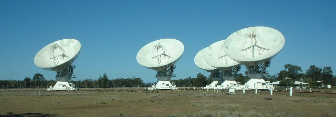
The ATCA is an array of six 22m diameter antennas located 237m above sea level at latitude -30° 18′ 46.385″ south, longitude 149° 33′ 00.500″ east. The array has a 3km east-west track with a 214m northern spur. Five antennas can be moved along these tracks, with the sixth antenna at a fixed position 3km to the west of the east-west track. The longest possible baseline is, therefore, 6km. The array can be used for observations in five wavelength bands between 27cm and (with five antennas only) 3mm, between frequencies of approximately 1.1GHz and 105GHz.
The location of six antennas at six stations is called an array configuration, or often, simply a configuration. The westernmost antenna, CA06, is fixed in position. The other five antennas can be positioned at any of 44 fixed stations. The station posts provide mains power to the antennas and network connections that allow commands from the control building to be sent to the antenna, and monitor data to be received from the antenna. The posts also have high-speed optical links that allow data from the antenna to be transferred to the control building. The smallest baseline increment available is 15.306m, and the shortest physical baseline is 30.612m. Five of the six ATCA antennas are shown in Figure 1.1.
A standard set of 17 configurations has been defined, and a subset of these is offered for each semester. These configurations have been designed to give optimum, minimum-redundancy coverage after a 12 hour observing period. Four configuration sets for the principal arrays (750m, 1.5km and 6km) are offered over several semesters (see Appendix H for details of these sets). Your choice of configuration depends on the extent, brightness and complexity of your source (see below).
The Australia Telescope Compact Array is an earth-rotation aperture synthesis radio interferometer. Earth-rotation aperture synthesis was first used in the 1950s for radio observations of the sun. The technique is comprehensively explained, with a historical perspective, in Interferometry and Synthesis in Radio Astronomy by Thompson, Moran & Swenson (Wiley, 3rd edition, 2017). Essentially, the array of antennas is comprised of a number of two-element interferometers. The visibility (i.e., the fraction of the signal common to both antennas of a pair) is derived by multiplying the (suitably delayed) signals together. By combining the correlated signals obtained over a long period of time and with a large range of spacings between antennas, the Compact Array measures the spatial coherence function:
where is the two dimensional intensity distribution on the sky, is the unit vector in the direction of the celestial source, is the separation vector between antennas 1 and 2 and indicates integration over the sphere (or, in practice, solid angle of the antenna beam).
The van Cittert–Zernike theorem states that the Fourier transformation of the spatial coherence function yields the source brightness distribution, i.e., the Fourier Transform of the visibilities produces an image of a radio source. The image is formed with the same angular resolution as for observations with a single antenna with a diameter equal to the largest spacing, however it will be less sensitive due to the interferometer's smaller collecting area.
By plotting the tracks that the baseline vectors trace out (from the source's perspective) as the Earth rotates, astronomers can gauge how good the telescope will be at imaging the source and resolving components in the field of view. This plot is referred to as the (u,v)-coverage as, by convention, the two orthogonal axes of the plot are u and v. These variables have units of the observing wavelength. The (u,v)-coverage shows where on the Fourier plane the image has been sampled.
To obtain the fullest (u,v) coverage with the ATCA would require observations with multiple different configurations, and for twelve hours with each configuration. However, almost any program can be successfully carried out with less than complete (u,v) coverage, and the individual configurations are chosen so as to optimise single configuration imaging characteristics. Sophisticated off-line image processing techniques minimise the effect of missing (u,v) coverage and allow reasonable images to be made with one configuration. For most programs, one to four configurations provide the best compromise between dynamic range, (u,v) coverage and time.
The smallest synthesized beamwidths in Right Ascension for each observing wavelength are shown in Table 1.1, but bear in mind that, for east-west arrays, the beamwidth in Declination is greater by a factor cosec(Dec). At high angular resolution, the telescope is only useful for observing southern objects. North of Declination -24°, full (u,v)-coverage is unobtainable; near Declination zero the beam is highly elongated north-south; and north of Declination +48° sources are below the telescope's +12° elevation limit and are inaccessible. For lower angular resolution, the north-south and hybrid arrays improve the (u,v)-coverage for equatorial sources, but only up to a maximum north-south baseline of 214m.
The rest of this chapter outlines the structure and operation of the ATCA. The path of the radio signal is traced through the system from the dish to the final data recording. This section is designed to help you understand how the Compact Array operates and provide all the information required to design an appropriate experiment. Detailed technical information about the ATCA can be found in the Journal of Electrical and Electronics Engineering, Australia, Special Issue, Vol. 12, No. 2, June 1992, a copy of which is available in the control room at the Narrabri Observatory.
The antennas have a Cassegrain design, i.e., the receivers are located in a turret that protrudes through the main reflector surface — see Figure 1.1. The antennas have an altitude-azimuth mount with wrap limits as shown in Figure 2.1. The shaped (i.e., non-parabolic) dish and subreflector surfaces are designed to maximise the gain to antenna noise ratio. The reflecting surface of antennas 1–5 are solid panels that allow observations up to 116 GHz. This is also true of the inner 15.3m of antenna 6. The outer reflecting surface of antenna 6 is made of perforated panels which permit observations at frequencies up to 50 GHz.
The subreflector mounted near the prime focus has a specially designed shape, differing slightly from the hyperbolic secondary of standard Cassegrain optics. The feedhorns are mounted on the optic axis — this allows polarisation measurements to be made, with very low ( ) instrumental polarisation. Subreflector height can be adjusted to achieve optimal focus for the different frequency bands. A major feature of the ATCA is its wide bandwidth operation. The feedhorns and front-end electronics operate over a very large range of frequencies, thus allowing (u,v) coverage to be increased by multi-frequency synthesis and dual frequency observations. The feedhorns are compact, with a corrugated interior surface and are designed for maximum frequency coverage, low noise, low spillover, low reflection and low cross-polarisation sidelobe levels. The feedhorns allow two simultaneous orthogonal linear polarisations to be measured (at frequencies almost an octave apart), and have a main lobe with near-constant, symmetrical beamwidth (James, G.L., 1984, IEEE Trans. Antennas Propagat. AP–22, pp 1134–1138; Thomas, B.M., James, G.L., Greene, K.J., 1986, IEEE Trans. Antennas Propagat. AP-34, pp 750–757).
The frequencies at which the Australia Telescope operates are listed in Table 1.1 see also section Section 1.3.1.
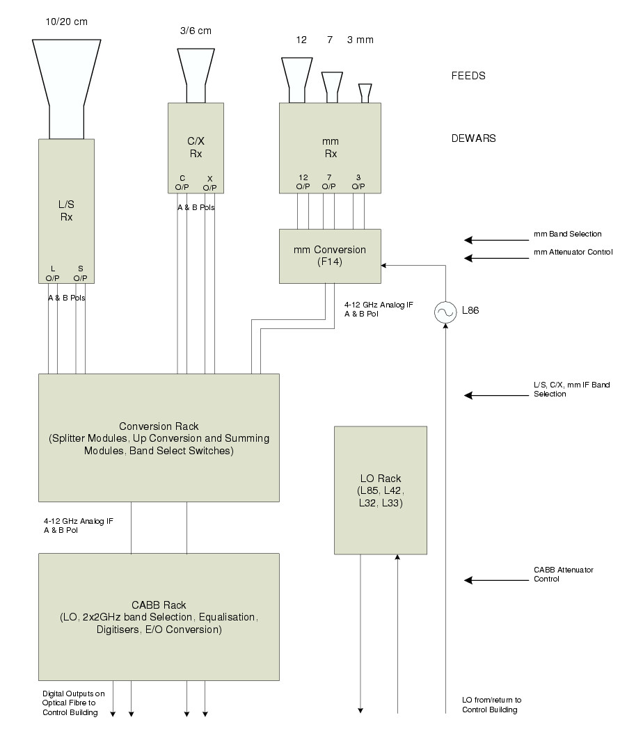
Each range of frequencies is referred to as a band. Bands are referred to by the wavelength of the approximate centre of the band or (especially at higher frequencies) by the frequency (and sometimes by the letter-codes shown over the columns of Table 1.1. There are presently five feedhorns mounted on each antenna (four on antenna 6): a large (2m high) feed-horn that operates in the 16cm band, and a somewhat smaller (50cm high) 4cm band feedhorn and three (several cm high) feedhorns mounted on the same dewar for the 15mm, 7mm and 3mm wavelengths. The feedhorns and the receivers are mounted on a rotating turret. The rotating turret design ensures that all feedhorns, when brought on-axis, are aligned with the optic axis of the antenna, allowing a wide field of view and dual-polarisation observations. The turrets are rotated automatically in accordance with the frequencies selected by the observing file. Rotating the turret orients the desired feed-horn and also ensures that the subsequent electronics suit the frequency at which you are observing. Changing the observing band to or from 7mm requires first rotating the turret to the 15mm position, and then translating the whole mm dewar to bring the 7mm feed on axis. The latter stage takes 2~3 minutes, and so changes to or from 7mm are much slower than any other band change.
Both the 16cm and 4cm band feedhorns are fitted with wide-bandwidth receivers that covers the horn's entire usable frequency range. All receivers run continuously and use cooled HEMT (high electron mobility transistor) and FET (field effect transistor) amplifiers that provide wide bandwidths and total system temperatures between 20K to 65K, depending on frequency.
The signals collected by the feedhorns are fed to the receiver systems for amplification and conversion to standard intermediate frequencies. During observations each antenna provides four independent intermediate frequency (IF) outputs (two frequency bands, two polarisations). These channels allow simultaneous observations of both polarisations at the two available frequencies in either dual-receiver system. The frequencies can be anywhere in the range covered by the selected feed-horn except at 15, 7 and 3mm where the two frequencies must be less than 6 GHz apart, and not straddle the 7mm sideband inversion (see Section 2.3.6).
In order to convert the received radio signals to lower frequencies, the radio signals are mixed with a “local oscillator" signal. Four local oscillator signals provide four IF outputs to enable the dual-frequency, dual-polarisation operation. You can also switch frequencies at the end of each integration cycle (typically ten seconds). To change to a pair of frequencies covered by a different feed-horn requires a rotation of the turret and takes about twenty seconds. However, to avoid excessive wear of the turrets, a limit of four rotations per hour is imposed. Thus time sharing between a number of frequencies is limited only by signal to noise ratio, wear and tear on the equipment, your imagination, and the off-line software.
The following sections describe the path of the signal from the initial reflection off the antenna surface, through to the data recorded onto export media, in more detail than the introduction above. Some radio-astronomy jargon is also explained, as is some important mathematics. The details of this section are not required by observers, but are included for completeness. A knowledge of the system is however essential if you want to design an experiment that uses the array in a new or unconventional way. Familiarity with the names and functions of some critical components can also be helpful if you need to diagnose faults. Many system components are housed in modules, and repairs can be made quickly by local staff replacing a module once a correct diagnosis has been made.
Radio waves (approximately within a range of 300 MHz to 120 GHz) are accurately reflected from the primary surface of the main parabolic dish and are re-reflected off a secondary reflector into a feed-horn. At the base of the feed-horn is a directional, coupling waveguide. In this coupler (the noise coupler) is a diode that injects a noise signal of known amplitude. This noise signal is used to calibrate the system temperature (Equation 1.1) and gain of the receiving system.
For radiation emitted by a randomly polarised source, the power received by a radio telescope is given by:
where A is the effective area of the antenna, S is the spectral power flux density and is the range of frequencies observed (the effective bandwidth). The factor of occurs because a detector can only respond to one polarisation component of the randomly polarised wave. The ATCA overcomes this limitation by providing separate detectors and electronics for two orthogonal polarisations, thus allowing all the power in the wave to be detected.
Table 1.1. Observing Parameters for the 6km Compact Array.
| Band Name | 16cm | 4cm | 15mm | 7mm | 3mm |
|---|---|---|---|---|---|
| Band Code | L / S | C / X | K | Q | W |
| Frequency Range (GHz) | 1.1 - 3.1 | 3.9 - 11.0 | 16 - 25 | 30 - 50 | 83 - 105 |
| Fractional frequency range | 95% | 95% | 44% | 50% | 24% |
| Number of antennas | 6 | 6 | 6 | 6 | 5 |
| Number of baselines | 15 | 15 | 15 | 15 | 10 |
| Primary beam [a] | 42′ - 15′ | 12′ - 4′ | 2′ | 70″ | 30″ |
| System temperature (K) [b] | 45 | 36 | 60 | 112 | 724 |
| System sensitivity (Jy) [c] | 55 | 43 | 72 | 136 | 1051 |
| Strongest confusing source (mJy) [d] | 140 - 24 | 2.3 - 0.4 | — | — | — |
| Array assumed below | 6 km | 6 km | 6 km | 6 km | H214 |
| Synthesized beam [e] | 9″ - 3″ | 3″ - 1″ | 0.5″ | 0.2″ | 2″ |
| Bandwidth assumed below (GHz) | 2 | 2 | 2 | 2 | 2 |
| Centre frequency assumed below (GHz) | 2.1 | 7.0 | 17.0 | 40.0 | 95.0 |
| Flux sensitivity (mJy/beam) (10 min) [f] | 0.04 | 0.03 | 0.05 | 0.09 | 0.70 |
| Brightness sensitivity (K) (10 min) [g] | 0.1 | 0.1 | 0.16 | 0.29 | 0.02 |
| Flux sensitivity (μJy/beam) (12 hr) | 4 | 3 | 5 | 33 | 83 |
| Brightness sensitivity (K) (12 hr) | 0.02 | 0.01 | 0.02 | 0.01 | 0.002 |
[a] Field of view (full width at half power). [b] The system temperature at high elevation under reasonable weather conditions. These values, particularly at high frequency, are weather-dependent. [c] The signal which doubles the system temperature. [d] Within FWHM primary beam — see A.H. Bridle, in Perley R.A., Schwab F.A. & Bridle A.H. (1989) “Synthesis Imaging in Radio Astronomy” Astron. Soc. Pacific Conf. Set., 6, p.471. [e] HPBW in R.A. for the 6 km array for all bands except 3mm, for which the H214 array is assumed. No taper applied. In Declination, for the 6 km array (and other pure east-west arrays), the HPBW is larger by cosec(Dec). Longer arrays (up to 3 km) are possible at 3mm but only with self-calibration and under favourable weather conditions. [f] Theoretical rms noise; one frequency; dual orthogonal polarisation; natural weighting. The effect of confusing sources can substantially degrade this number. This is the 1σ Gaussian-noise level. [g] For the array listed in the same column: see following table for shorter arrays. This is the 1σ Gaussian-noise level. | |||||
The sensitivity of a radio telescope is the minimum signal power that can be distinguished from the random fluctuations at the output of the receiving system which are caused by noise inherent in the system. The sensitivity is usually defined as the spectral power flux density of a source that would produce the same signal power as the noise power. It is measured in Jansky (Jy), with
The noise power consists of two main components: the noise power due to the receiving amplifier and other electrical system components, and the noise due to ground radiation, thermal emission from the atmosphere (which varies with elevation, cloud cover, etc.), background radio emission from our Galaxy and other sources detected by the antenna. These noise powers are usually referred to as equivalent temperatures, although at no point is a physical temperature measured. The “temperature” due to the noise power is called the system temperature, , and is related to the noise power by:
where
is the noise power and
is Boltzmann's constant. As both the source and noise signals are random
in nature, measurements of the power levels made at time intervals
separated by
can be considered independent
(e.g., Thompson, Moran & Swenson 1986, 2001). If the signal level is
averaged for
seconds then
samples have been measured.
The signal to noise ratio is the ratio of the power in the output that is due to the radio source being observed to that caused by the noise, and is given by:
In this expression, is the antenna temperature, the equivalent temperature of the radio source being observed. Note that “antenna temperature" is sometimes also taken to mean the contribution to the noise power from radio noise detected by the antenna, as described above. For typical values for bandwidth (2 GHz) and integration time (12 hours), it is possible to detect a signal for which the power level is less than times the noise level.
The noise source in the noise coupler injects a signal that is about 5% of the level of the system temperature at a rate of 8 Hz. This noise signal is synchronously demodulated and the following relationship holds:
Here,
is the equivalent temperature of the noise
source,
is the power received while the noise diode is
on, and
is the power received while the noise diode is
off.
is measured accurately once by placing a thermal
radiator of known temperature (a microwave absorber at 300K, giving
300K
)
directly above the feeds. The power received
with this load in place is then compared with the power output with
the antenna just looking at the sky (
).
This measurement is used to establish the level of
,
which is assumed not to vary with time. The measurement of system and antenna
temperature is described in a
technical memo by
Sinclair and Gough (1991). And despite our assumption that this level should not
vary with time, it can be calibrated by the correlator at any time using a point source
with a known flux density, with the acal command
(Section 3.3.6.4).
The noise coupler is mounted on another coupler that provides a vacuum seal between the noise coupler and the subsequent receiver system, which is housed in an evacuated, cryogenic cylinder. An air gap thermally isolates the cylinder, the contents of which are cooled by a helium pump to 20K. The second coupler is mounted on the polariser. The dual function of the polariser is to select the two linear polarisations and the desired band, so it is also known as a band splitter. The polariser consists of four strips of metal inside a conical waveguide that “guide” two orthogonal linear polarisations into probes at the narrow end of the polariser. The way in which the metal strips select the linear polarisations can be thought of as analogous to the effect of a ridged waveguide, which constrains a particular mode to propagate along the region between the ridge and the roof of the waveguide. The probes are simply short (with respect to the wavelength) lengths of the cores of the coaxial cables that take the signal into the first amplifiers. Thus the polariser converts a wave into a voltage: the impedance of the circuit is effectively the same as a waveguide impedance, so it works like a well-matched load. The polariser's official title is quad-ridged orthomode transducer, or OMT. Separate electronics exist for both orthogonal linear polarisations, which are measured simultaneously. The position angle of the polariser is fixed with respect to the antenna. As the antennas have altitude-azimuth mounts, the position angle of the linear probes rotate on the sky during the course of an observation (imagine a circumpolar line on the sky orbiting around a stationary antenna). Measurement of both polarisations is therefore required for polarised sources. The two linear polarisations can be combined to give an accurate total intensity: the Stokes I parameter. Without additional calibration, the other Stokes parameters (the linear polarisation measures Q, and U, and the circularly polarised component V) can be in error by about 2% of the value of I. Measurements of the phase difference of the two linear polarisations (referred to as the X and Y (or A and B) polarisations) at the receiver by on-line hardware may need further off-line calibration.
For an unpolarised source, observing both orthogonal polarisations offers a improvement in signal to noise ratio for an I image over an image generated from only one polarisation.
The signal is taken from the feedhorn into a low noise, broadband amplifier.
The receivers each use two low-noise amplifiers (LNAs) to amplify the signal by 30–40 dB. All six antennas are fitted with wideband, continuously running, receivers. Cooled indium-phosphide high electron mobility transistors (InP HEMTs) are used at 16cm and 4cm, and indium-phosphide monolithic microwave integrated circuit (InP MMIC) devices are used at 15mm, 7mm and 3mm. Only the “inner" five antennas (i.e., excluding CA06) have 3mm receivers. The accessible frequency range is given in Table 1.1, and the average system temperatures are given in Table 1.4 and in Section 1.3.1. Note that frequencies outside these nominal limits may be accessible.
The next step is the conversion to the frequency range that is used by the CABB digitisers. The 4cm signals require no conversion, whereas the mm signals require a down-conversion stage, and the 16cm signals require up-conversion to the 4 to 12 GHz band.
The local oscillator signals have a relatively narrow tuning range, lying in the regions between the radio frequency bands (this reduces the likelihood of self-generated interference).
The final output from the conversion system is sent to the samplers for digitisation. The CABB (Compact Array Broadband Backend) samplers were developed in-house and are capable of 4 gigasamples per second (GS/s), with 10 bit sampling (more information is available in the February 2007 ATNF newsletter and in Wilson et al. (2011, MNRAS, 416, 832)).
The samplers, which are also referred to as the CABB digitisers, do two things. First the analog (continuously variable in time and amplitude) signal is sampled into a discrete-time sequence of values. This process does not degrade the signal as it is sampled at the Nyquist rate (twice the inverse frequency of the bandwidth of the analog signal). Subsequently, each of the discrete-time, continuously variable values are converted to one of a finite set of values: this is called quantising. CABB uses 9-bit sampling (internally, as stated above, 10-bit sampling is used, with 9 bits transferred to the correlator), with approximately 6-bits used in sampling the regular data range, and the additional bits providing extra robustness in the case of interference RFI (radio-frequency interference). The digitised signals from the sampler are sent from each antenna to the correlator along optic fibres at a rate of 160 gigabits per second for each antenna. Optical fibres run from the samplers in each antenna to the correlator, which is housed in the screened room (to prevent RFI generated by the correlator electronics from affecting the observations) of the central control building. Synchronising code is added to the data stream at the start of each integration cycle to allow each bit to be correctly identified at the correlator irrespective of temporal changes in the length of the fibre.
The correlator effectively multiplies simultaneous signals from two samplers: the more similar the signal from both antennas, the larger the degree of correlation. A plane wavefront approaching the ATCA will, in general, arrive at different antennas at different times. The signals from the antennas therefore need to be delayed before being presented to the correlator so as to simulate a wavefront arriving at each antenna simultaneously. This was previously achieved by separate delay units, but is now included in the CABB boards. The delay calibration undertaken at the start of an observation removes other delays caused by return path length differences, instrumental delay variations and the like, so that wavefront samples are presented to the correlator synchronously.
The CABB filterbank/correlator is divided across a number of Digital Signal Processing (DSP) boards. The DSP boards use Virtex-4 Xilinx Field Programmable Gated Arrays (FPGAs) to provide a flexible, programmable hardware correlator. The output from the correlator is averaged for the period of one integration cycle, and sent to the correlator control computer caccc where it is written to hard disk. Integration cycles can be set by the observer, between 2 and 30 seconds, although the default cycle time of 10 seconds is generally recommended for all observers. (For mosaic-mode observations, 6-seconds is the practical minimum cycle time.)
More information on the correlator can be found at the CABB webpage.
The CABB correlator provides a number of observing modes:
Two always-available 2048 MHz continuum IF bands (although an analogue bandpass filter may reduce the usable bandwidth by 32 MHz). These can currently be divided into 2048 x 1MHz channels or 32 x 64MHz channels, with up to 16 “zoom” bands able to be placed for higher spectral resolution.
Up to 6 GHz separation of simultaneous IF centre frequencies (depending on receiver restrictions)
9 bit sampling accuracy
Square, independent channels (ie. no leakage between channels)
All polarisation parameters for all products (including auto-correlations)
Up to 16 zoom bands per IF to provide finer spectral resolution
A pulsar binning mode
This design ensures that the user will always get high continuum sensitivity from the wide-bandwidth IFs, while providing very high spectral resolution for line studies at the same time.